pyoptim
1.0.0
Pyoptim:用於優化和矩陣操作的Python軟件包
該項目是Ensias的數值分析與優化課程的一個組成部分,Mohammed v University源於M. Naoum教授的建議,即創建一個python包裝,封裝了實驗室會議期間實踐的算法。它重點介紹了大約十種不受限制的優化算法,提供2D和3D可視化,從而可以在計算效率和準確性方面進行性能比較。此外,該項目涵蓋了矩陣操作,例如反轉,分解和求解線性系統,所有這些都集成在包含實驗室衍生算法的軟件包中。
GIF來源:https://www.nsf.gov/news/mmg/mmg/mmg_disp.jsp?med_id = 78950&from=]
該項目的每個部分都是示例代碼,該代碼顯示瞭如何執行以下操作:
實現單變量優化算法,encompassing fixed_step,Accelerated_step,Enternive_search,dichotomous_search,Interval_halving,fibonacci,fibonacci,golden_section,golden_section,armijo_backward和armijo_forward。
摻入各種單變量優化算法,包括梯度下降,梯度共軛,牛頓,Quasi_newton_dfp,隨機梯度下降。
2D,輪廓和3D格式中所有算法的每個迭代步驟的可視化。
進行比較分析,重點是其運行時和準確性指標。
矩陣操作的實施,例如反轉(例如,高斯 - 約旦),分解(例如,LU,Choleski)和線性系統的解決方案(例如,高斯 - 約旦,LU,Choleski)。
安裝此Python軟件包:
pip install pyoptim運行此演示筆記本
 import pyoptim . my_scipy . onevar_optimize . minimize as soom
import pyoptim . my_plot . onevar . _2D as po2 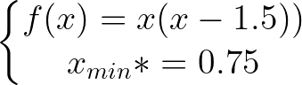
 def f ( x ):
return x * ( x - 1.5 ) # analytically, argmin(f) = 0.75 
 xs = - 10
xf = 10
epsilon = 1.e-2 print ( 'x* =' , soom . fixed_step ( f , xs , epsilon ))
po2 . fixed_step ( f , xs , epsilon ) x* = 0.75 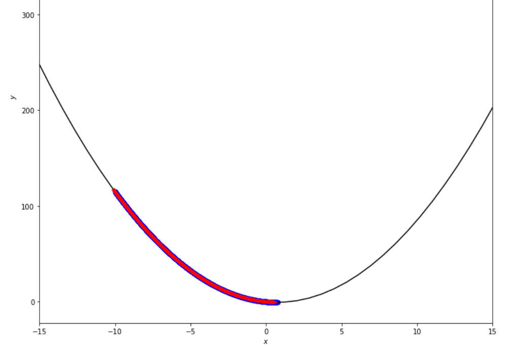
達到最小值之前,固定步驟算法採取的步驟順序
 print ( 'x* =' , soom . accelerated_step ( f , xs , epsilon ))
po2 . accelerated_step ( f , xs , epsilon )
x* = 0.86 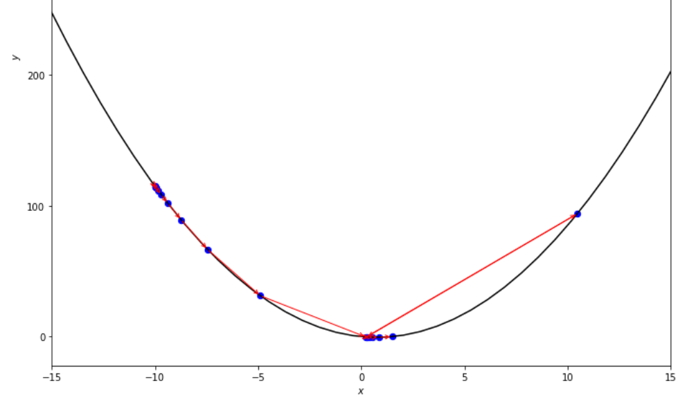
在達到最小值之前,加速步驟算法採取的步驟順序
 print ( 'x* =' , soom . exhaustive_search ( f , xs , xf , epsilon ))
po2 . exhaustive_search ( f , xs , xf , epsilon )
x* = 0.75
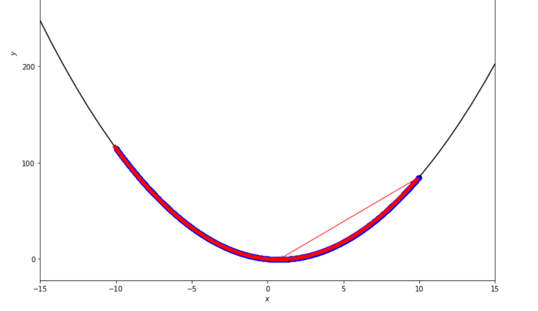
到達最小值之前,詳盡的搜索算法採取的步驟順序
 mini_delta = 1.e-3
print ( 'x* =' , soom . dichotomous_search ( f , xs , xf , epsilon , mini_delta ))
po2 . dichotomous_search ( f , xs , xf , epsilon , mini_delta )
x* = 0.7494742431640624
達到最小值之前,二分法搜索算法採取的步驟順序
 print ( 'x* =' , soom . interval_halving ( f , xs , xf , epsilon ))
po2 . interval_halving ( f , xs , xf , epsilon )
x* = 0.75
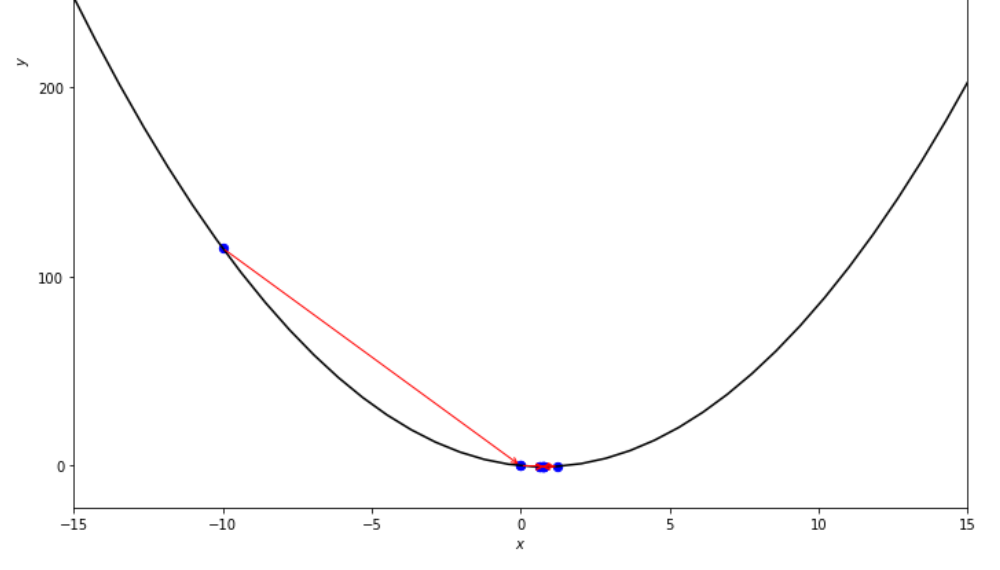
在達到最小值之前,間隔將算法減半的步驟序列。
 n = 15
print ( 'x* =' , soom . fibonacci ( f , xs , xf , n ))
po2 . fibonacci ( f , xs , xf , n )
x* = 0.76 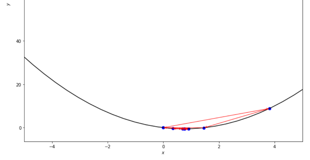
在達到最小值之前,斐波那契算法採取的步驟順序。
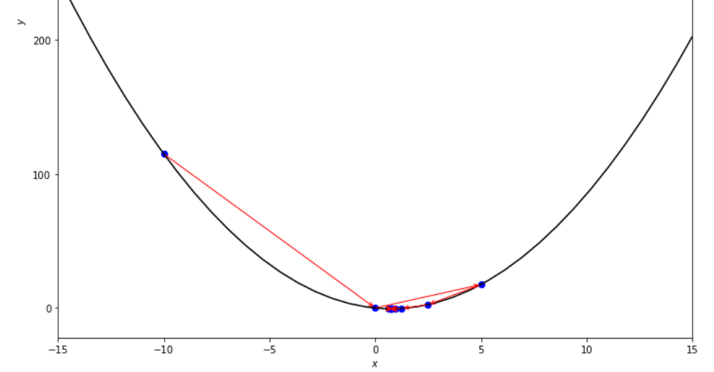
 print ( 'x* =' , soom . golden_section ( f , xs , xf , epsilon ))
po2 . golden_section ( f , xs , xf , epsilon )
x* = 0.75 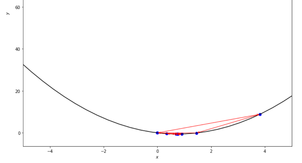
達到最小值之前,黃金部分算法採取的步驟順序
 ŋ = 2
xs = 100
print ( 'x* =' , soom . armijo_backward ( f , xs , ŋ , epsilon ))
po2 . armijo_backward ( f , xs , ŋ , epsilon )
x* = 0.78 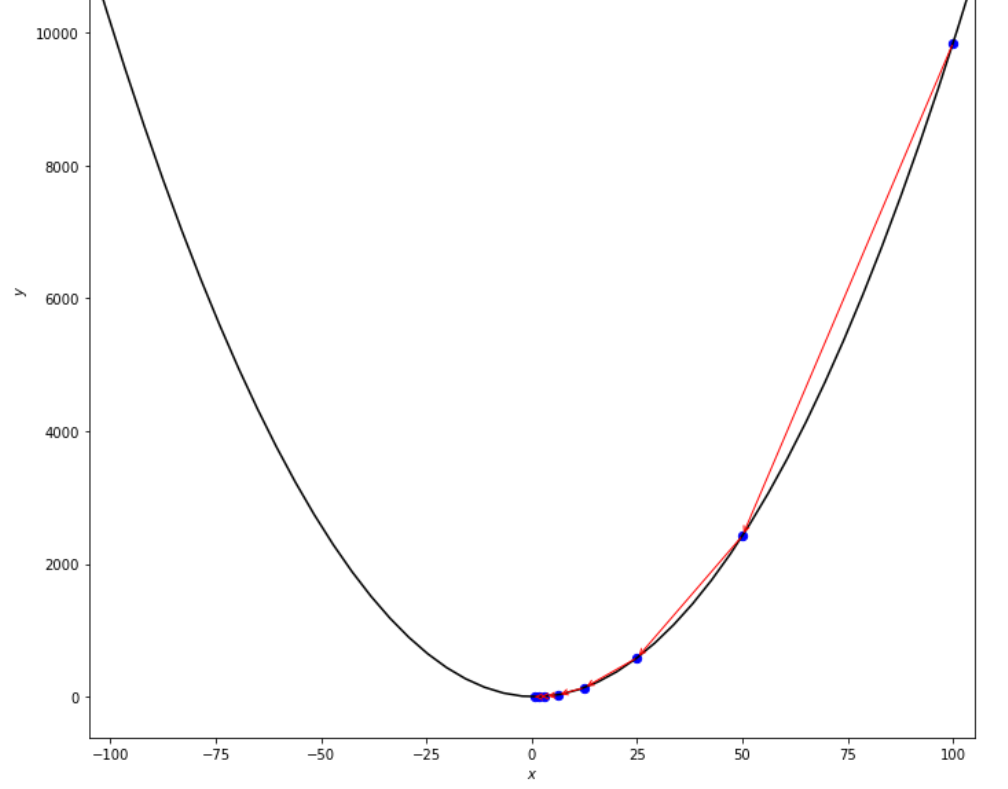
在達到最小值之前,Armijo向後算法採取的步驟順序
 xs = 0.1
epsilon = 0.5
ŋ = 2
print ( 'x* =' , soom . armijo_forward ( f , xs , ŋ , epsilon ))
po2 . armijo_forward ( f , xs , ŋ , epsilon )
x* = 0.8 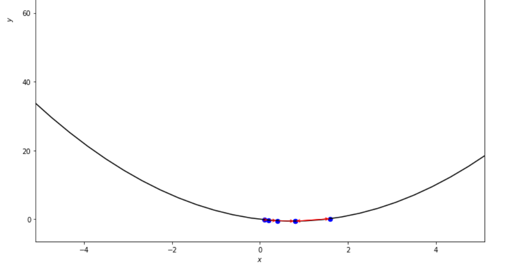
在達到最小值之前,Armijo前進算法採取的步驟順序
po2 . compare_all_time ( f , 0 , 2 , 1.e-2 , 1.e-3 , 10 , 2 , 0.1 , 100 )運行時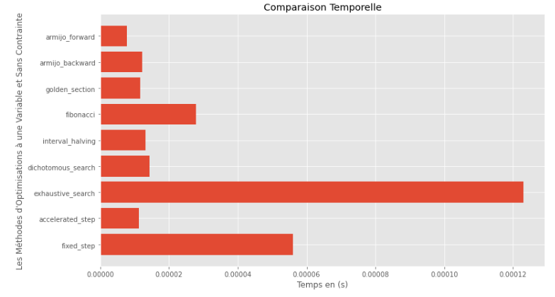
po2 . compare_all_precision ( f , 0 , 2 , 1.e-2 , 1.e-3 , 10 , 2 , 0.1 , 100 )真實和計算最小值之間的差距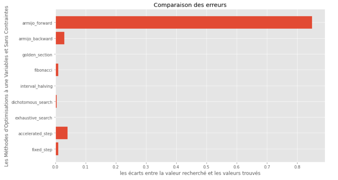
從運行時和精度圖可以推斷出,在該凸單動函數評估的算法中,金段方法作為最佳選擇而出現,提供了高精度和尤其是較低的運行時的融合。
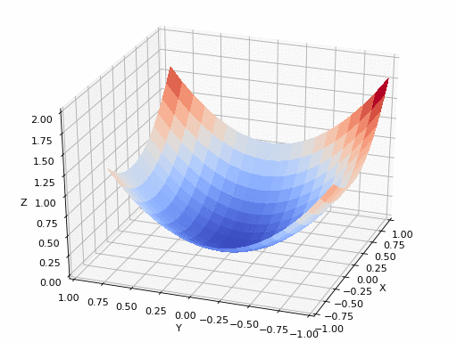
 import pyoptim . my_plot . multivar . _3D as pm3
import pyoptim . my_plot . multivar . contour2D as pmc def h ( x ):
return x [ 0 ] - x [ 1 ] + 2 * ( x [ 0 ] ** 2 ) + 2 * x [ 1 ] * x [ 0 ] + x [ 1 ] ** 2
# analytically, argmin(f) = [-1, 1.5]分類解決方案
 X = [ 1000 , 897 ]
alpha = 1.e-2
tol = 1.e-2 pmc . gradient_descent ( h , X , tol , alpha )
pm3 . gradient_descent ( h , X , tol , alpha ) Y* = [-1.01 1.51]達到最小值之前,梯度下降算法採取的步驟順序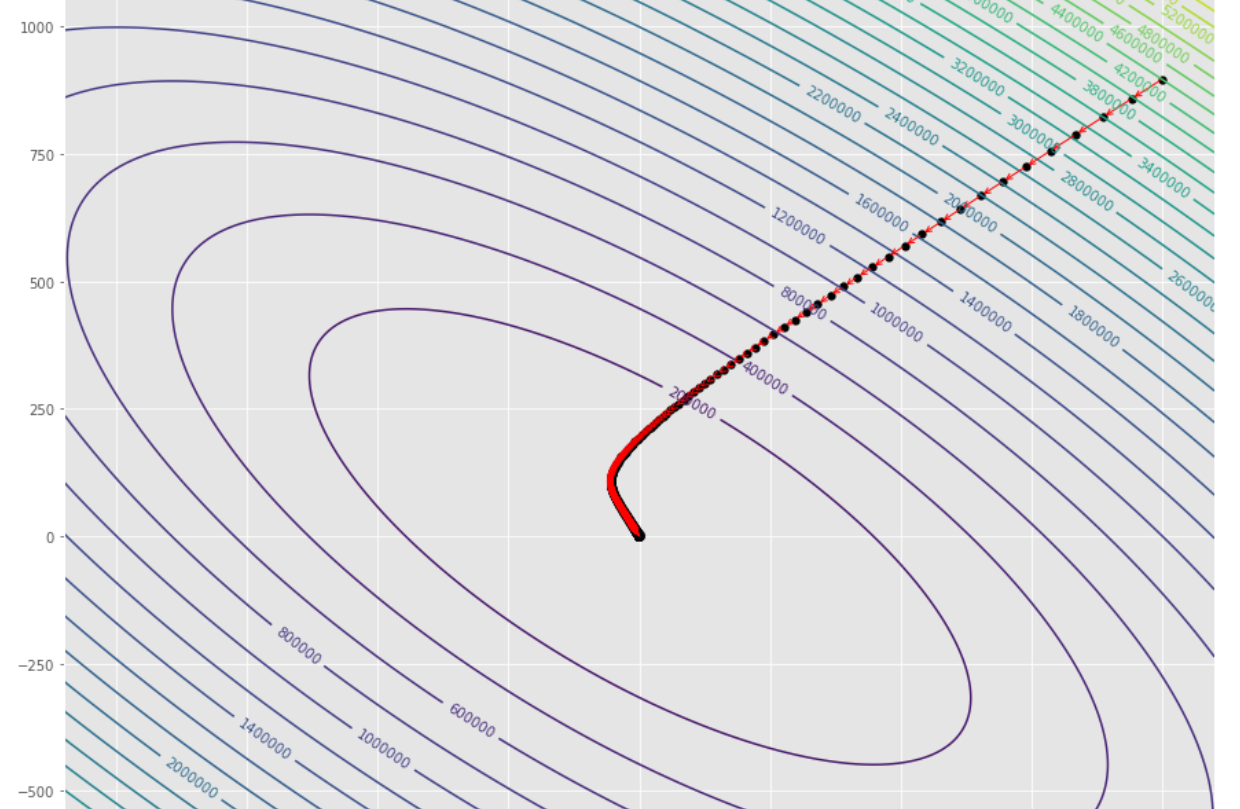
輪廓圖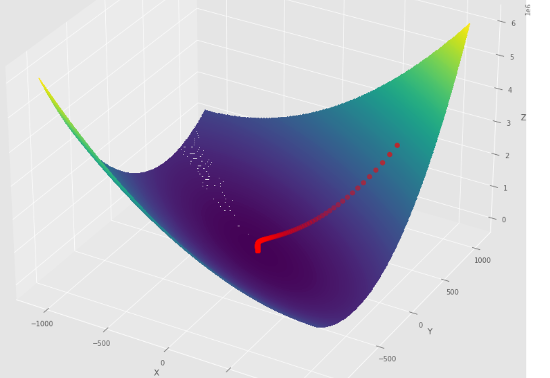
3D圖
 pmc . gradient_conjugate ( h , X , tol )
pm3 . gradient_conjugate ( h , X , tol )
Y* = [-107.38 172.18]達到最小值之前,梯度共軛算法採取的步驟順序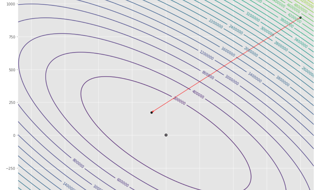
輪廓圖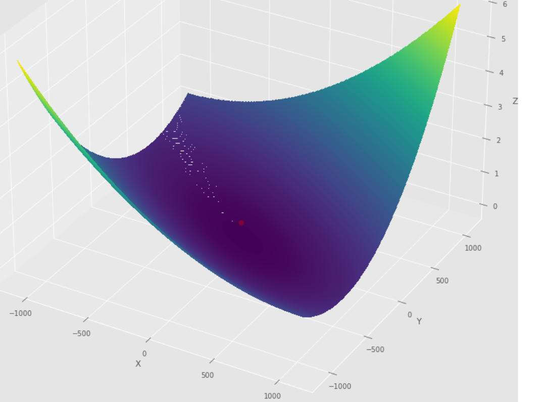
3D圖
 pmc . newton ( h , X , tol )
pm3 . newton ( h , X , tol )
Y* = [-1. 1.5]達到最小值之前,牛頓算法採取的步驟順序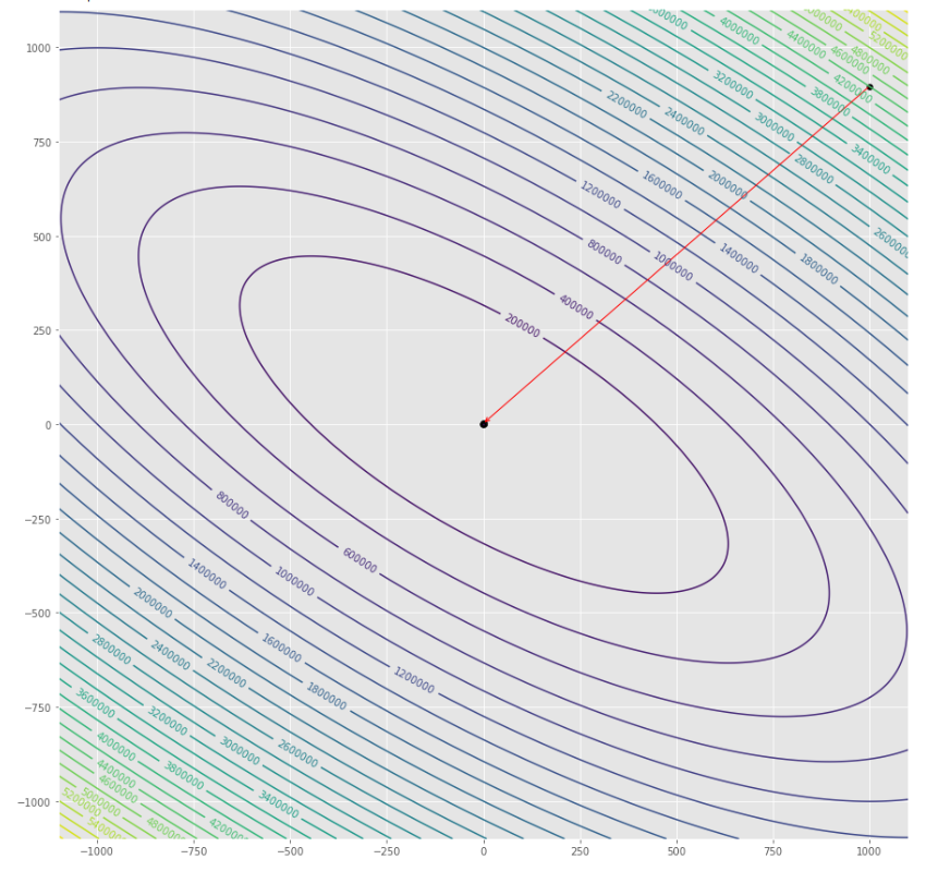
輪廓圖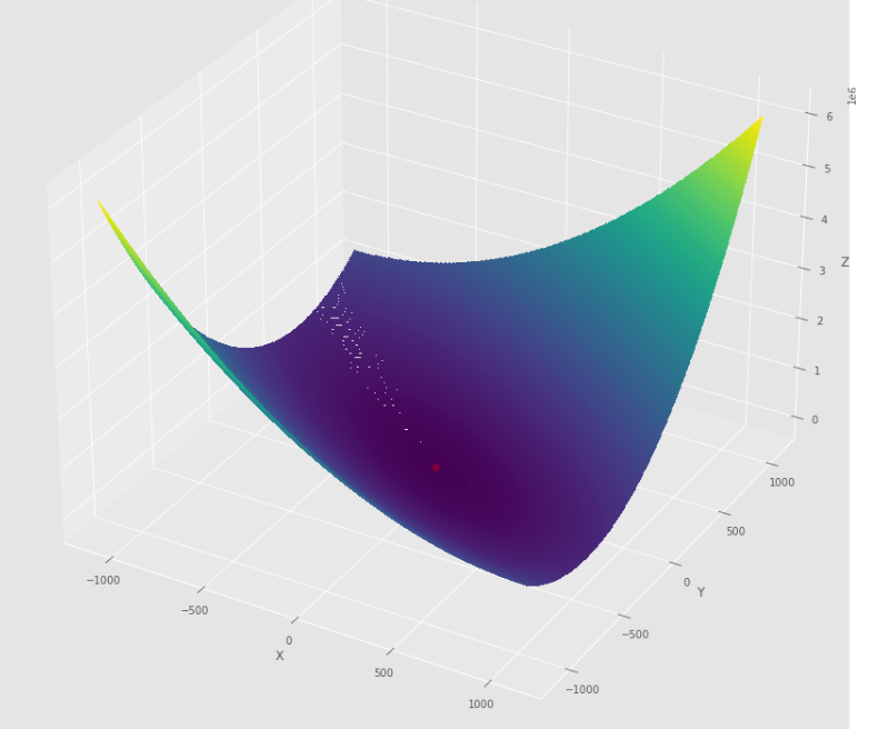
3D圖
 pmc . quasi_newton_dfp ( h , X , tol )
pm3 . quasi_newton_dfp ( h , X , tol )
Y* = [-1. 1.5]準牛頓DFP算法採取的步驟順序,然後達到最低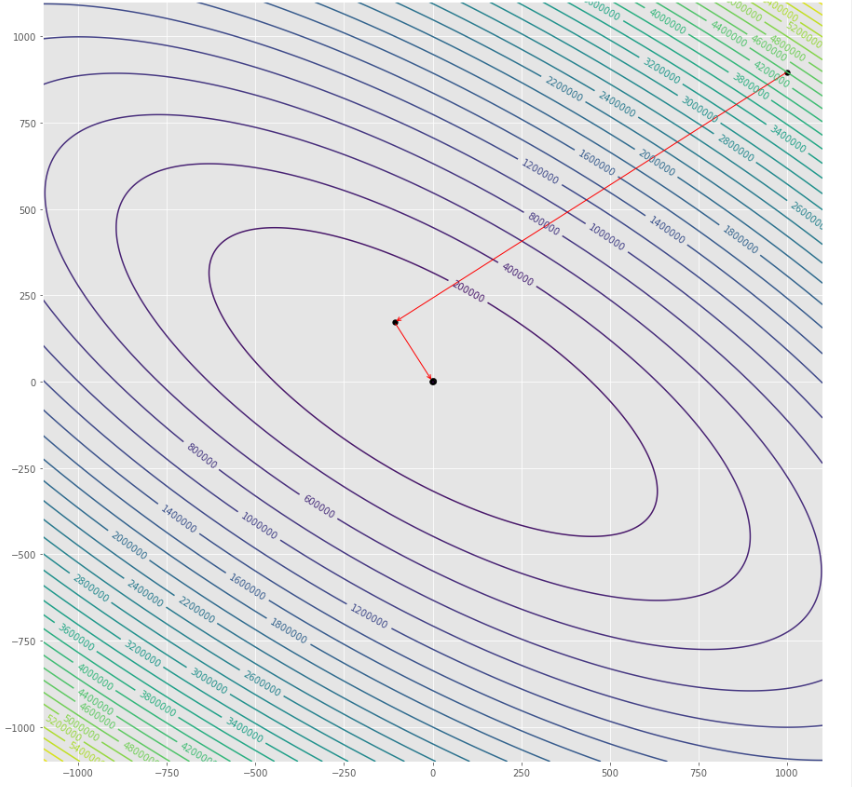
輪廓圖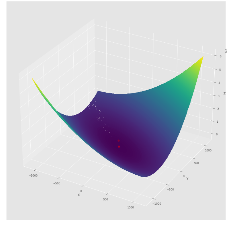
3D圖
 pmc . sgd ( h , X , tol , alpha )
pm3 . sgd ( h , X , tol , alpha )
Y* = [-1.01 1.52]在達到最小值之前,由隨機梯度下降算法採取的步驟順序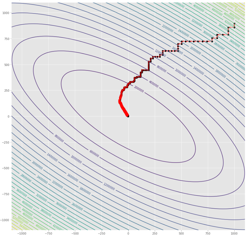
輪廓圖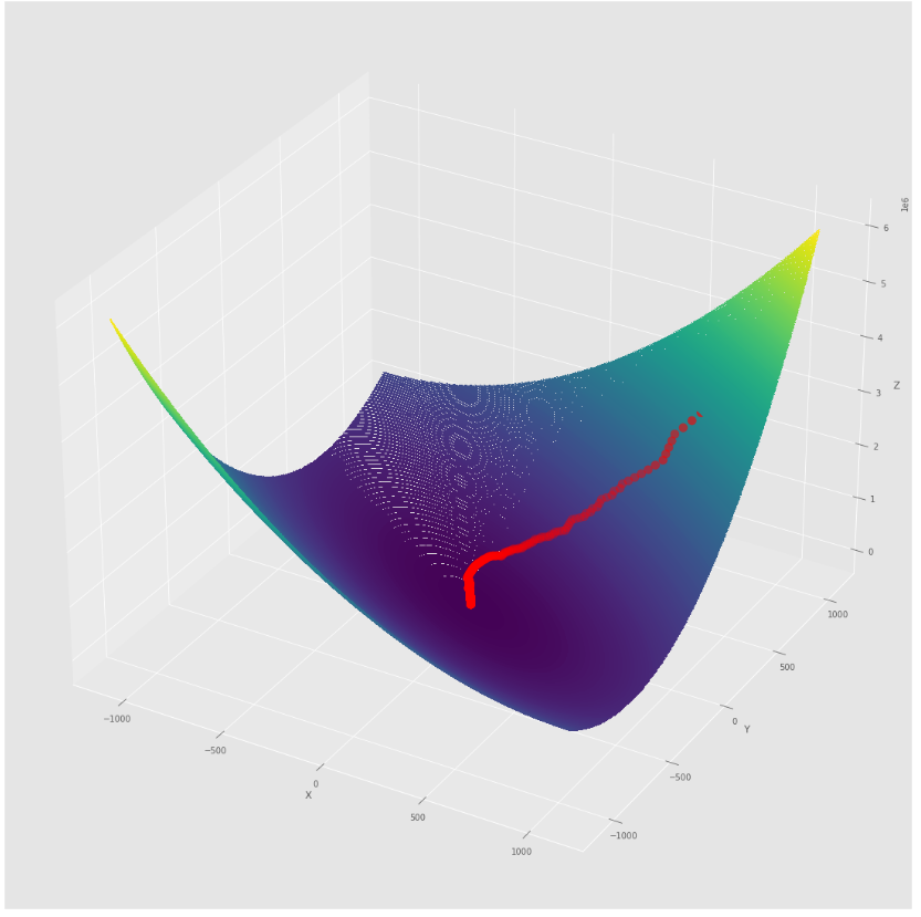
3D圖
 alpha = 100 #it must be high because of BLS
c = 2
pmc . sgd_with_bls ( h , X , tol , alpha , c )
pm3 . sgd_with_bls ( h , X , tol , alpha , c )
Y* = [-1. 1.5]在達到最小值之前,由隨機梯度下降採取的步驟順序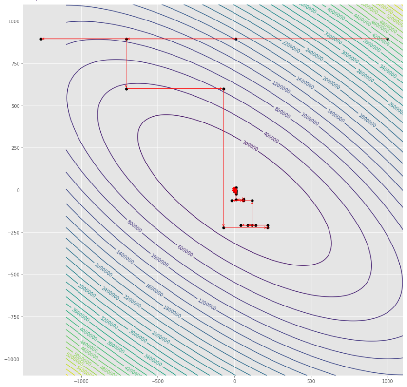
輪廓圖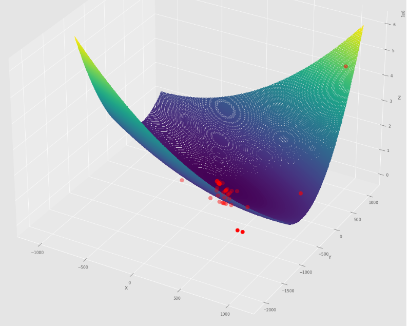
3D圖
pm3 . compare_all_time ( h , X , 1.e-2 , 1.e-1 , 100 , 2 )運行時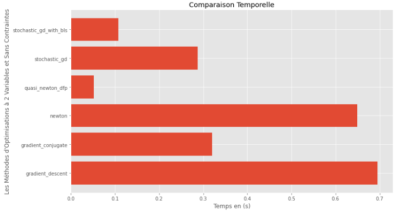
pm3 . compare_all_precision ( h , X , 1.e-2 , 1.e-1 , 100 , 2 )真實和計算最小值之間的差距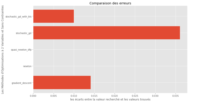
從運行時和精度圖可以推斷出,在該凸多變量函數評估的算法中,準牛頓DFP方法作為最佳選擇而出現,提供了高精度和尤其是低運行時的融合。
import pyoptim . my_numpy . inverse as npi 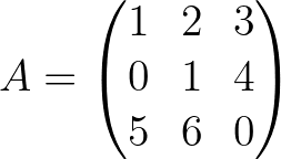
A = np . array ([[ 1. , 2. , 3. ],[ 0. , 1. , 4. ],[ 5. , 6. , 0. ]]) A_1 = npi . gaussjordan ( A . copy ())
I = A @ A_1
I = np . around ( I , 1 )
print ( 'A_1 = n n ' , A_1 )
print ( ' n A_1*A = n n ' , I ) A_1 =
[[-24. 18. 5.]
[ 20. -15. -4.]
[ -5. 4. 1.]]
A_1*A =
[[1. 0. 0.]
[0. 1. 0.]
[0. 0. 1.]] import pyoptim . my_numpy . decompose as npd A = np . array ([[ 1. , 2. , 3. ],[ 0. , 1. , 4. ],[ 5. , 6. , 0. ]]) #A is not positive definite
B = np . array ([[ 2. , - 1. , 0. ],[ - 1. , 2. , - 1. ],[ 0. , - 1. , 2. ]]) #B is positive definite
Y = np . array ([ 45 , - 78 , 95 ]) #randomly chosen column vector L , U , P = npd . LU ( A )
print ( "P = n " , P , " n n L = n " , L , " n n U = n " , U )
print ( " n " , A == P @ L @ U ) P =
[[0. 0. 1.]
[0. 1. 0.]
[1. 0. 0.]]
L =
[[1. 0. 0. ]
[0. 1. 0. ]
[0.2 0.8 1. ]]
U =
[[ 5. 6. 0. ]
[ 0. 1. 4. ]
[ 0. 0. -0.2]]
[[ True True True]
[ True True True]
[ True True True]] L = npd . choleski ( A ) # A is not positive definite
print ( L )
print ( "--------------------------------------------------" )
L = npd . choleski ( B ) # B is positive definite
print ( 'L = n ' , L , ' n ' )
C = np . around ( L @( L . T ), 1 )
print ( 'B = L@(L.T) n n ' , B == C ) A must be positive definite !
None
--------------------------------------------------
L =
[[ 1.41421356 0. 0. ]
[-0.70710678 1.22474487 0. ]
[ 0. -0.81649658 1.15470054]]
B = L@(L.T)
[[ True True True]
[ True True True]
[ True True True]] import pyoptim . my_numpy . solve as nps 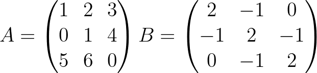
 A = np . array ([[ 1. , 2. , 3. ], [ 0. , 1. , 4. ], [ 5. , 6. , 0. ]]) # A is not positive definite
B = np . array ([[ 2. , - 1. , 0. ], [ - 1. , 2. , - 1. ], [ 0. , - 1. , 2. ]]) # B is positive definite
Y = np . array ([ 45 , - 78 , 95 ]) # randomly chosen column vector X = nps . gaussjordan ( A , Y )
print ( "X = n " , X )
print ( " n A@X=Y n " , A @ X == Y , ' n ' )
print ( '---------------------------------------------------------------' )
X = nps . gaussjordan ( B , Y )
print ( "X = n " , X )
Y_ = np . around ( B @ X , 1 )
print ( " n B@X=Y n " , Y_ == Y , ' n ' ) X =
[[-2009.]
[ 1690.]
[ -442.]]
A@X=Y
[[ True]
[ True]
[ True]]
---------------------------------------------------------------
X =
[[18.5]
[-8. ]
[43.5]]
B@X=Y
[[ True]
[ True]
[ True]]
 X = nps . LU ( A , Y )
print ( "X* = n " , X )
print ( " n AX*=Y n " , A @ X == Y )
print ( "-------------------------------------------------------------------------------" );
X = nps . LU ( B , Y )
print ( "X* = n " , X )
Y_ = np . around ( B @ X , 1 )
print ( " n BX*=Y n " , Y_ == Y )
X* =
[[-2009.]
[ 1690.]
[ -442.]]
AX*=Y
[[ True]
[ True]
[ True]]
-------------------------------------------------------------------------------
X* =
[[18.5]
[-8. ]
[43.5]]
BX*=Y
[[ True]
[ True]
[ True]] X = nps . choleski ( A , Y )
print ( "-------------------------------------------------------------------------------" )
X = nps . choleski ( B , Y )
print ( "X = n " , X )
Y_ = np . around ( B @ X , 1 )
print ( " n BX*=Y n " , Y_ == Y ) !! A must be positive definite !!
-------------------------------------------------------------------------------
X =
[[18.5]
[-8. ]
[43.5]]
BX*=Y
[[ True]
[ True]
[ True]]

