pyoptim
1.0.0
Pyoptim: Paket Python untuk Operasi Optimasi dan Matriks
Proyek ini, komponen dari kursus analisis & optimasi numerik di ENINSIAS, Universitas Mohammed V muncul dari saran Profesor M. Naoum untuk membuat paket Python yang merangkum algoritma yang dipraktikkan selama sesi laboratorium. Ini berfokus pada sekitar sepuluh algoritma optimasi yang tidak dibatasi, menawarkan visualisasi 2D dan 3D, memungkinkan perbandingan kinerja dalam efisiensi dan akurasi komputasi. Selain itu, proyek ini mencakup operasi matriks seperti inversi, dekomposisi, dan pemecahan sistem linier, semua terintegrasi dalam paket yang berisi algoritma yang diturunkan dari lab.
Sumber GIF: https://www.nsf.gov/news/mmg/mmg_disp.jsp?med_id=78950&from= media(https://aria42.com/blog/2014/12/understanding-lbfgs
Setiap bagian dari proyek ini adalah kode sampel yang menunjukkan cara melakukan hal berikut:
Implementasi algoritma optimisasi satu variabel, meliputi Fixed_Step, Accelerated_Step, Light_search, Dichotomous_Search, Interval_halving, Fibonacci, Golden_Section, Armijo_backward, dan Armijo_forward.
Penggabungan berbagai algoritma optimasi satu variabel, termasuk keturunan gradien, konjugat gradien, Newton, quasi_newton_dfp, keturunan gradien stokastik.
Visualisasi setiap langkah iterasi untuk semua algoritma dalam format 2D, kontur, dan 3D.
Melakukan analisis komparatif yang berfokus pada runtime dan metrik akurasi mereka.
Implementasi operasi matriks seperti inversi (misalnya, Gauss-Jordan), dekomposisi (misalnya, Lu, Choleski), dan solusi untuk sistem linier (misalnya, Gauss-Jordan, Lu, Choleski).
Untuk menginstal paket Python ini:
pip install pyoptimJalankan buku catatan demo ini
 import pyoptim . my_scipy . onevar_optimize . minimize as soom
import pyoptim . my_plot . onevar . _2D as po2 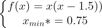
 def f ( x ):
return x * ( x - 1.5 ) # analytically, argmin(f) = 0.75 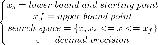
 xs = - 10
xf = 10
epsilon = 1.e-2 print ( 'x* =' , soom . fixed_step ( f , xs , epsilon ))
po2 . fixed_step ( f , xs , epsilon ) x* = 0.75 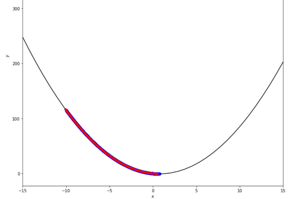
Urutan langkah yang diambil oleh algoritma langkah tetap sebelum mencapai minimum
 print ( 'x* =' , soom . accelerated_step ( f , xs , epsilon ))
po2 . accelerated_step ( f , xs , epsilon )
x* = 0.86 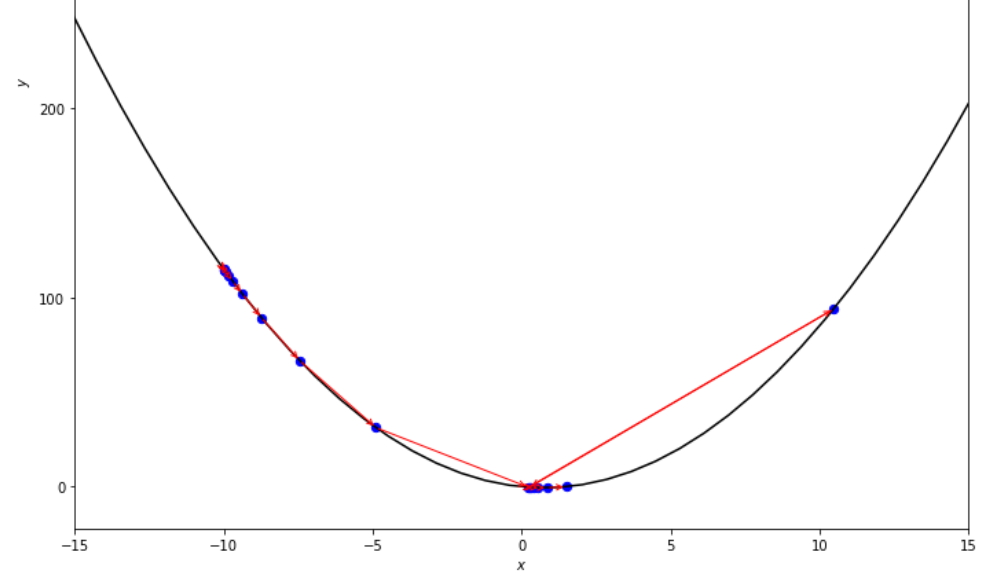
Urutan langkah yang diambil oleh algoritma langkah yang dipercepat sebelum mencapai minimum
 print ( 'x* =' , soom . exhaustive_search ( f , xs , xf , epsilon ))
po2 . exhaustive_search ( f , xs , xf , epsilon )
x* = 0.75
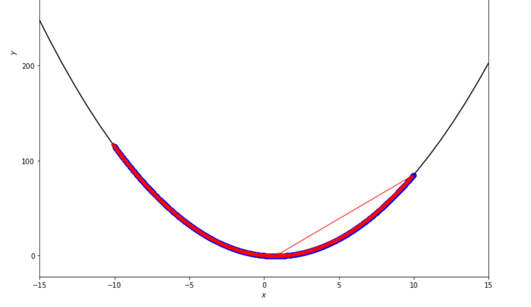
Urutan langkah yang diambil oleh algoritma pencarian lengkap sebelum mencapai minimum
 mini_delta = 1.e-3
print ( 'x* =' , soom . dichotomous_search ( f , xs , xf , epsilon , mini_delta ))
po2 . dichotomous_search ( f , xs , xf , epsilon , mini_delta )
x* = 0.7494742431640624
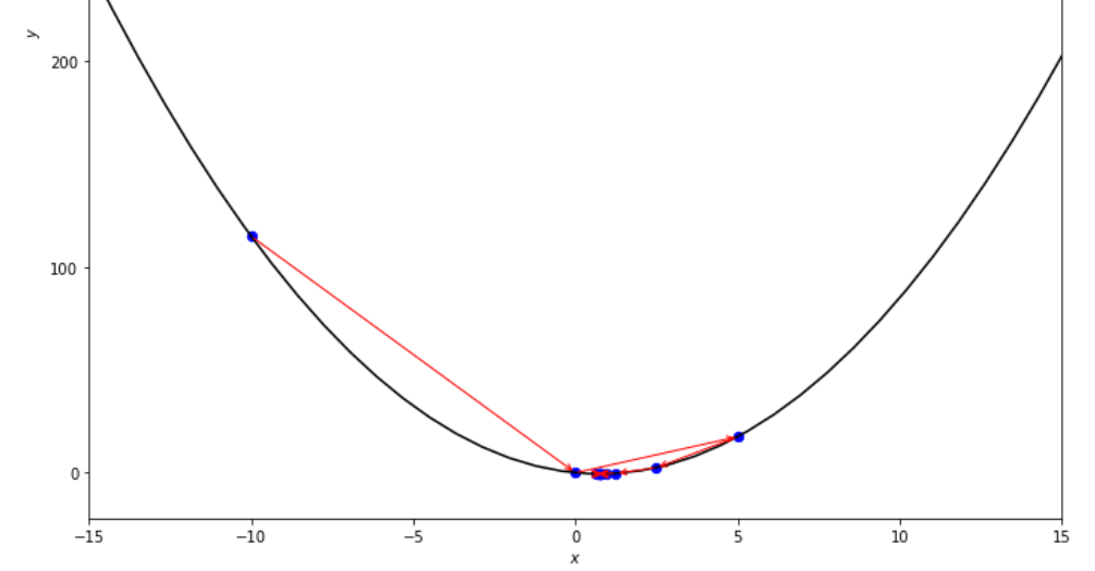
Urutan langkah yang diambil oleh algoritma pencarian dikotomis sebelum mencapai minimum
 print ( 'x* =' , soom . interval_halving ( f , xs , xf , epsilon ))
po2 . interval_halving ( f , xs , xf , epsilon )
x* = 0.75
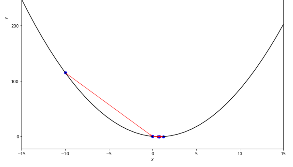
Urutan langkah yang diambil oleh algoritma separuh interval sebelum mencapai minimum.
 n = 15
print ( 'x* =' , soom . fibonacci ( f , xs , xf , n ))
po2 . fibonacci ( f , xs , xf , n )
x* = 0.76 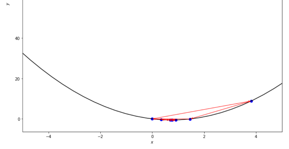
Urutan langkah yang diambil oleh algoritma Fibonacci sebelum mencapai minimum.
 print ( 'x* =' , soom . golden_section ( f , xs , xf , epsilon ))
po2 . golden_section ( f , xs , xf , epsilon )
x* = 0.75 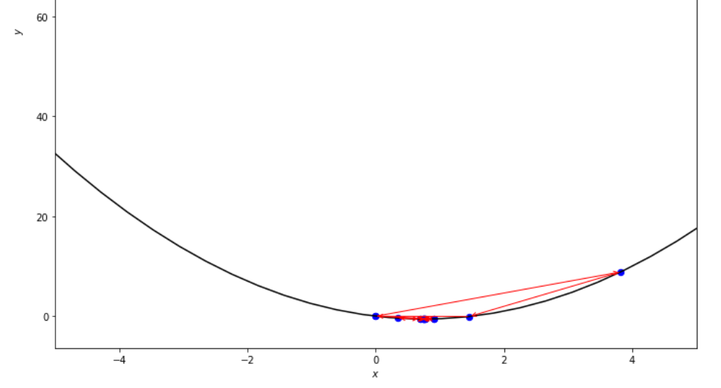
Urutan langkah yang diambil oleh algoritma bagian emas sebelum mencapai minimum
 ŋ = 2
xs = 100
print ( 'x* =' , soom . armijo_backward ( f , xs , ŋ , epsilon ))
po2 . armijo_backward ( f , xs , ŋ , epsilon )
x* = 0.78 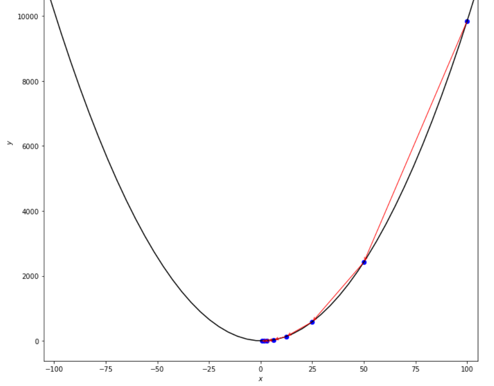
Urutan langkah yang diambil oleh algoritma mundur Armijo sebelum mencapai minimum
 xs = 0.1
epsilon = 0.5
ŋ = 2
print ( 'x* =' , soom . armijo_forward ( f , xs , ŋ , epsilon ))
po2 . armijo_forward ( f , xs , ŋ , epsilon )
x* = 0.8 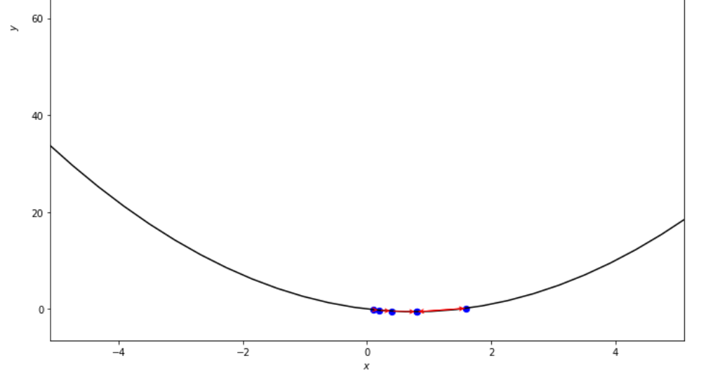
Urutan langkah -langkah yang diambil oleh algoritma Forward Armijo sebelum mencapai minimum
po2 . compare_all_time ( f , 0 , 2 , 1.e-2 , 1.e-3 , 10 , 2 , 0.1 , 100 ) Runtime 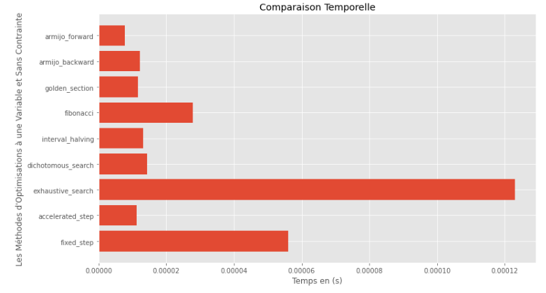
po2 . compare_all_precision ( f , 0 , 2 , 1.e-2 , 1.e-3 , 10 , 2 , 0.1 , 100 ) Kesenjangan antara minimum yang benar dan yang dihitung 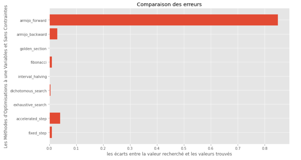
Dari runtime dan grafik akurasi, dapat disimpulkan bahwa di antara algoritma yang dinilai untuk fungsi variabel tunggal cembung ini, metode bagian emas muncul sebagai pilihan optimal, menawarkan perpaduan akurasi tinggi dan runtime yang sangat rendah.
 import pyoptim . my_plot . multivar . _3D as pm3
import pyoptim . my_plot . multivar . contour2D as pmc def h ( x ):
return x [ 0 ] - x [ 1 ] + 2 * ( x [ 0 ] ** 2 ) + 2 * x [ 1 ] * x [ 0 ] + x [ 1 ] ** 2
# analytically, argmin(f) = [-1, 1.5]solusi analitikal
 X = [ 1000 , 897 ]
alpha = 1.e-2
tol = 1.e-2 pmc . gradient_descent ( h , X , tol , alpha )
pm3 . gradient_descent ( h , X , tol , alpha ) Y* = [-1.01 1.51] Urutan langkah yang diambil oleh algoritma keturunan gradien sebelum mencapai minimum 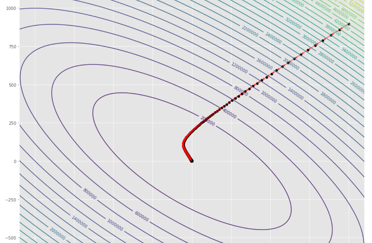
Plot kontur 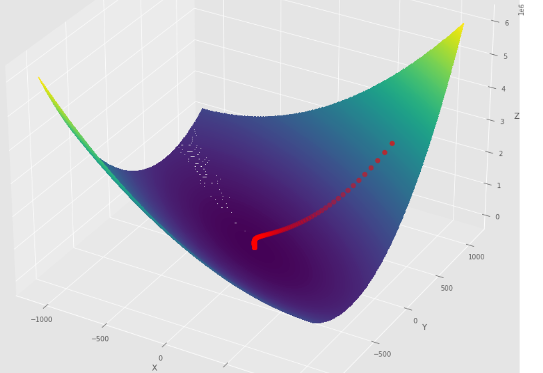
Plot 3D
 pmc . gradient_conjugate ( h , X , tol )
pm3 . gradient_conjugate ( h , X , tol )
Y* = [-107.38 172.18] Urutan langkah yang diambil oleh algoritma konjugat gradien sebelum mencapai minimum 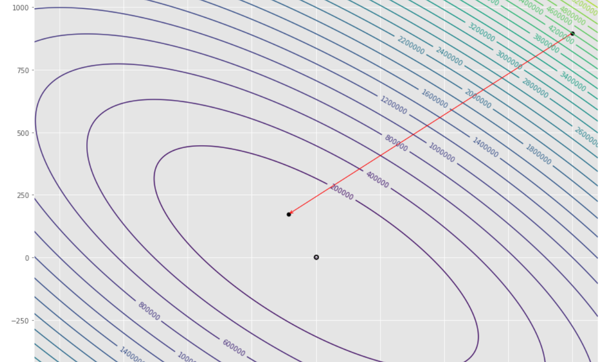
Plot kontur 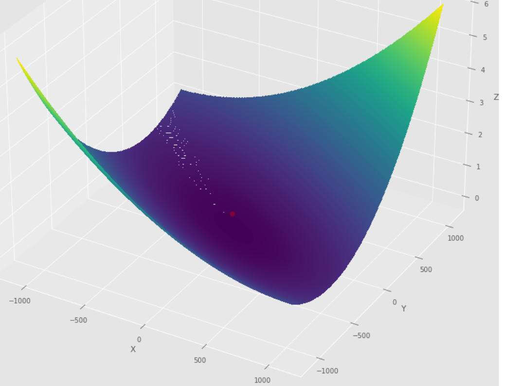
Plot 3D
 pmc . newton ( h , X , tol )
pm3 . newton ( h , X , tol )
Y* = [-1. 1.5] Urutan langkah yang diambil oleh algoritma Newton sebelum mencapai minimum 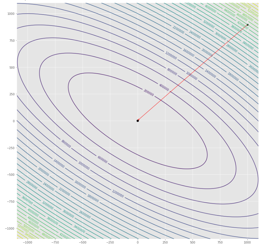
Plot kontur 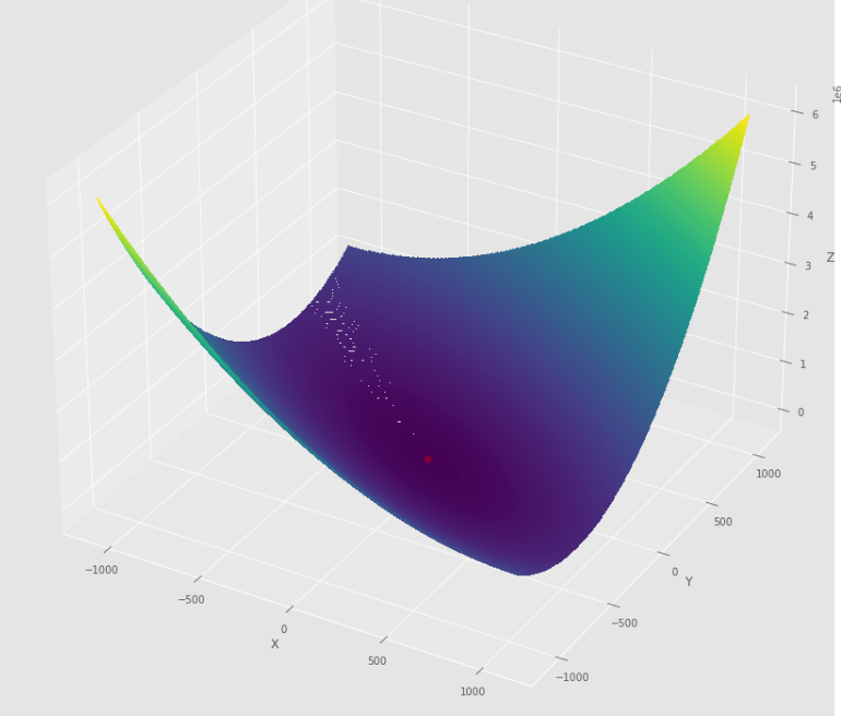
Plot 3D
 pmc . quasi_newton_dfp ( h , X , tol )
pm3 . quasi_newton_dfp ( h , X , tol )
Y* = [-1. 1.5] Urutan langkah yang diambil oleh algoritma quasi newton dfp sebelum mencapai minimum 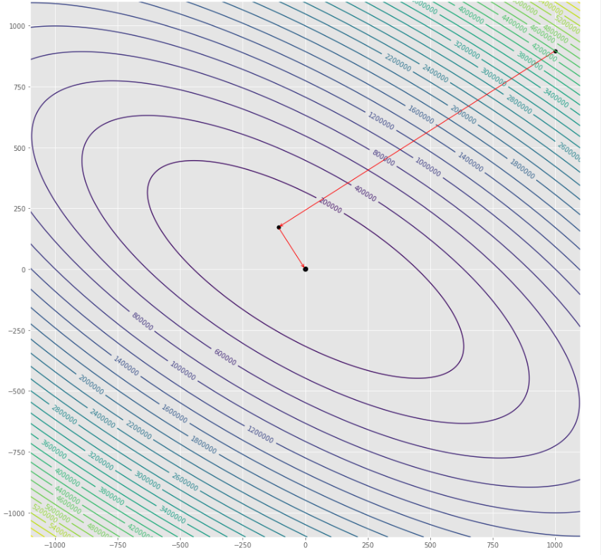
Plot kontur 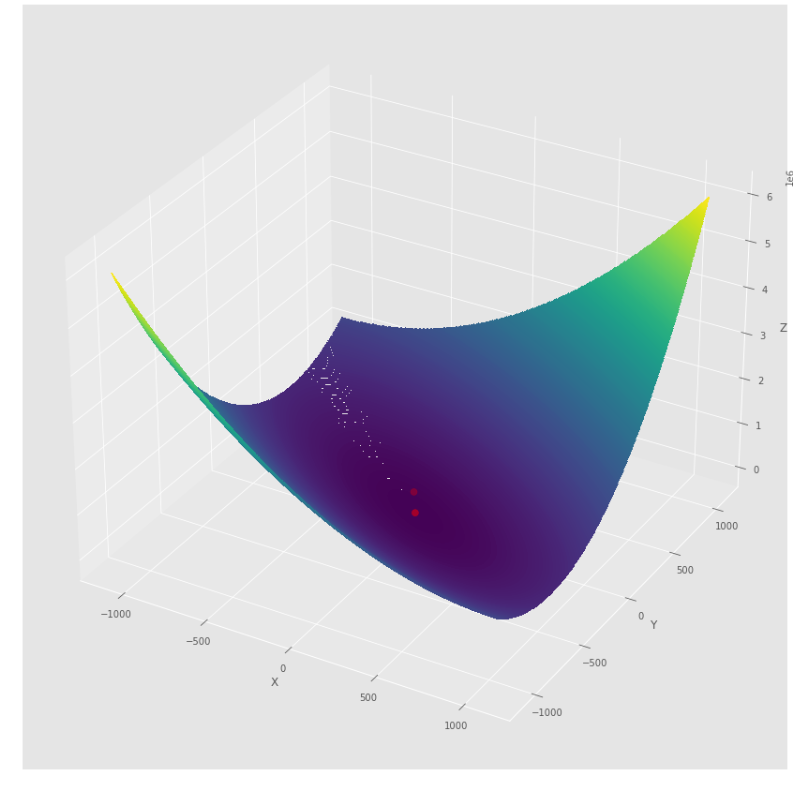
Plot 3D
 pmc . sgd ( h , X , tol , alpha )
pm3 . sgd ( h , X , tol , alpha )
Y* = [-1.01 1.52] Urutan langkah yang diambil oleh algoritma keturunan gradien stokastik sebelum mencapai minimum 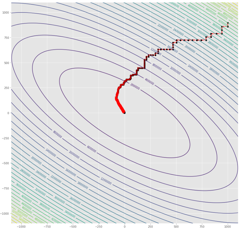
Plot kontur 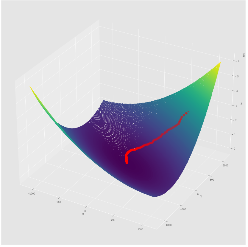
Plot 3D
 alpha = 100 #it must be high because of BLS
c = 2
pmc . sgd_with_bls ( h , X , tol , alpha , c )
pm3 . sgd_with_bls ( h , X , tol , alpha , c )
Y* = [-1. 1.5] Urutan langkah yang diambil oleh keturunan gradien stokastik dengan algoritma BLS sebelum mencapai minimum 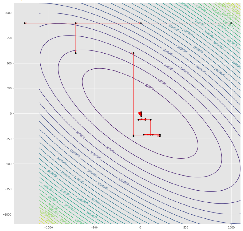
Plot kontur 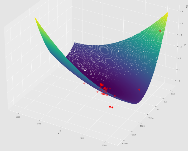
Plot 3D
pm3 . compare_all_time ( h , X , 1.e-2 , 1.e-1 , 100 , 2 ) Runtime 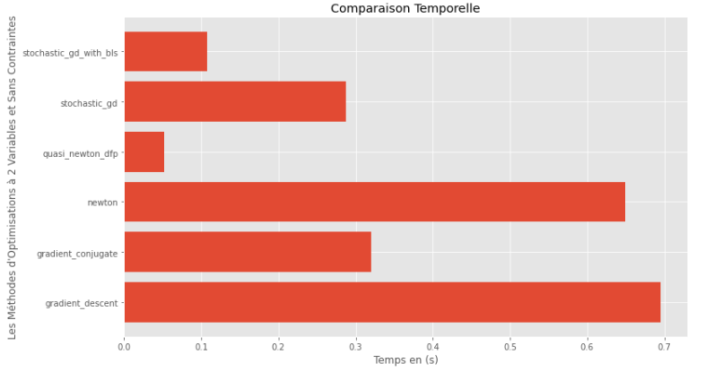
pm3 . compare_all_precision ( h , X , 1.e-2 , 1.e-1 , 100 , 2 ) Kesenjangan antara minimum yang benar dan yang dihitung 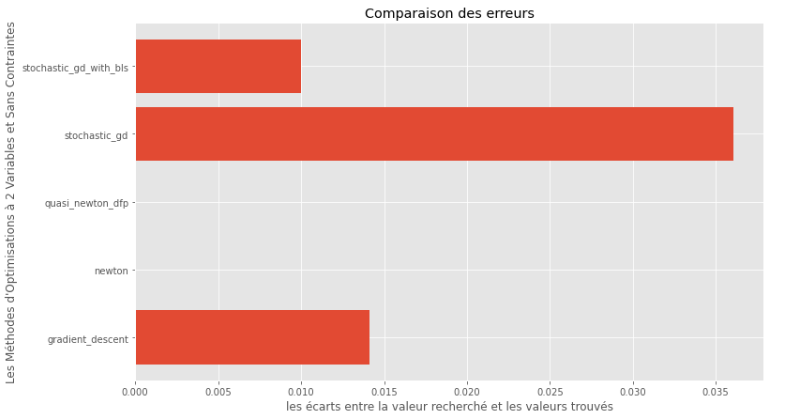
Dari runtime dan grafik akurasi, dapat disimpulkan bahwa di antara algoritma yang dinilai untuk fungsi multivariabel cembung ini, metode kuasi Newton DFP muncul sebagai pilihan optimal, menawarkan perpaduan akurasi tinggi dan runtime rendah.
import pyoptim . my_numpy . inverse as npi 
A = np . array ([[ 1. , 2. , 3. ],[ 0. , 1. , 4. ],[ 5. , 6. , 0. ]]) A_1 = npi . gaussjordan ( A . copy ())
I = A @ A_1
I = np . around ( I , 1 )
print ( 'A_1 = n n ' , A_1 )
print ( ' n A_1*A = n n ' , I ) A_1 =
[[-24. 18. 5.]
[ 20. -15. -4.]
[ -5. 4. 1.]]
A_1*A =
[[1. 0. 0.]
[0. 1. 0.]
[0. 0. 1.]] import pyoptim . my_numpy . decompose as npd A = np . array ([[ 1. , 2. , 3. ],[ 0. , 1. , 4. ],[ 5. , 6. , 0. ]]) #A is not positive definite
B = np . array ([[ 2. , - 1. , 0. ],[ - 1. , 2. , - 1. ],[ 0. , - 1. , 2. ]]) #B is positive definite
Y = np . array ([ 45 , - 78 , 95 ]) #randomly chosen column vector L , U , P = npd . LU ( A )
print ( "P = n " , P , " n n L = n " , L , " n n U = n " , U )
print ( " n " , A == P @ L @ U ) P =
[[0. 0. 1.]
[0. 1. 0.]
[1. 0. 0.]]
L =
[[1. 0. 0. ]
[0. 1. 0. ]
[0.2 0.8 1. ]]
U =
[[ 5. 6. 0. ]
[ 0. 1. 4. ]
[ 0. 0. -0.2]]
[[ True True True]
[ True True True]
[ True True True]] L = npd . choleski ( A ) # A is not positive definite
print ( L )
print ( "--------------------------------------------------" )
L = npd . choleski ( B ) # B is positive definite
print ( 'L = n ' , L , ' n ' )
C = np . around ( L @( L . T ), 1 )
print ( 'B = L@(L.T) n n ' , B == C ) A must be positive definite !
None
--------------------------------------------------
L =
[[ 1.41421356 0. 0. ]
[-0.70710678 1.22474487 0. ]
[ 0. -0.81649658 1.15470054]]
B = L@(L.T)
[[ True True True]
[ True True True]
[ True True True]] import pyoptim . my_numpy . solve as nps 
 A = np . array ([[ 1. , 2. , 3. ], [ 0. , 1. , 4. ], [ 5. , 6. , 0. ]]) # A is not positive definite
B = np . array ([[ 2. , - 1. , 0. ], [ - 1. , 2. , - 1. ], [ 0. , - 1. , 2. ]]) # B is positive definite
Y = np . array ([ 45 , - 78 , 95 ]) # randomly chosen column vector X = nps . gaussjordan ( A , Y )
print ( "X = n " , X )
print ( " n A@X=Y n " , A @ X == Y , ' n ' )
print ( '---------------------------------------------------------------' )
X = nps . gaussjordan ( B , Y )
print ( "X = n " , X )
Y_ = np . around ( B @ X , 1 )
print ( " n B@X=Y n " , Y_ == Y , ' n ' ) X =
[[-2009.]
[ 1690.]
[ -442.]]
A@X=Y
[[ True]
[ True]
[ True]]
---------------------------------------------------------------
X =
[[18.5]
[-8. ]
[43.5]]
B@X=Y
[[ True]
[ True]
[ True]]
 X = nps . LU ( A , Y )
print ( "X* = n " , X )
print ( " n AX*=Y n " , A @ X == Y )
print ( "-------------------------------------------------------------------------------" );
X = nps . LU ( B , Y )
print ( "X* = n " , X )
Y_ = np . around ( B @ X , 1 )
print ( " n BX*=Y n " , Y_ == Y )
X* =
[[-2009.]
[ 1690.]
[ -442.]]
AX*=Y
[[ True]
[ True]
[ True]]
-------------------------------------------------------------------------------
X* =
[[18.5]
[-8. ]
[43.5]]
BX*=Y
[[ True]
[ True]
[ True]] X = nps . choleski ( A , Y )
print ( "-------------------------------------------------------------------------------" )
X = nps . choleski ( B , Y )
print ( "X = n " , X )
Y_ = np . around ( B @ X , 1 )
print ( " n BX*=Y n " , Y_ == Y ) !! A must be positive definite !!
-------------------------------------------------------------------------------
X =
[[18.5]
[-8. ]
[43.5]]
BX*=Y
[[ True]
[ True]
[ True]]

