SimplestSimulatedAnnealing
1.0.0
การใช้งานที่ง่ายที่สุด (จาก DPEA) ของวิธีการหลอมจำลอง
pip install SimplestSimulatedAnnealing
นี่คืออัลกอริทึมวิวัฒนาการสำหรับ การลดฟังก์ชั่น
ขั้นตอน:
f ต้องย่อให้เล็กสุดx0 (สามารถสุ่ม)mut ฟังก์ชั่นนี้ควรให้โซลูชันใหม่ (สามารถสุ่ม) x1 โดยใช้ข้อมูลเกี่ยวกับ x0 และอุณหภูมิ Tcooling (พฤติกรรมอุณหภูมิ)Tx0 และคะแนนที่ดีที่สุด f(x0)x1 = mut(x0) และคำนวณ f(x1)f(x1) < f(x0) เราพบวิธีแก้ปัญหาที่ดีกว่า x0 = x1 มิฉะนั้นเราสามารถแทนที่ x1 ด้วย x0 ด้วยความน่าจะเป็นเท่ากับ exp((f(x0) - f(x1)) / T)T โดยใช้ฟังก์ชั่นการระบาย cooling : T = cooling(T)นำเข้าแพ็คเกจ:
 import math
import numpy as np

from SimplestSimulatedAnnleaning import SimulatedAnnealing , Cooling , simple_continual_mutation
กำหนดฟังก์ชั่นย่อ (rastrigin):
 def Rastrigin ( arr ):
    return 10 * arr . size + np . sum ( arr ** 2 ) - 10 * np . sum ( np . cos ( 2 * math . pi * arr ))

dim = 5
เราจะใช้การกลายพันธุ์แบบเกาส์ที่ง่ายที่สุด:
mut = simple_continual_mutation ( std = 0.5 )สร้างวัตถุโมเดล (ชุดฟังก์ชันและมิติ):
model = SimulatedAnnealing ( Rastrigin , dim )เริ่มค้นหาและดูรายงาน:
 best_solution , best_val = model . run (
    start_solution = np . random . uniform ( - 5 , 5 , dim ),
    mutation = mut ,
    cooling = Cooling . exponential ( 0.9 ),
    start_temperature = 100 ,
    max_function_evals = 1000 ,
    max_iterations_without_progress = 100 ,
    step_for_reinit_temperature = 80
    )

model . plot_report ( save_as = 'simple_example.png' )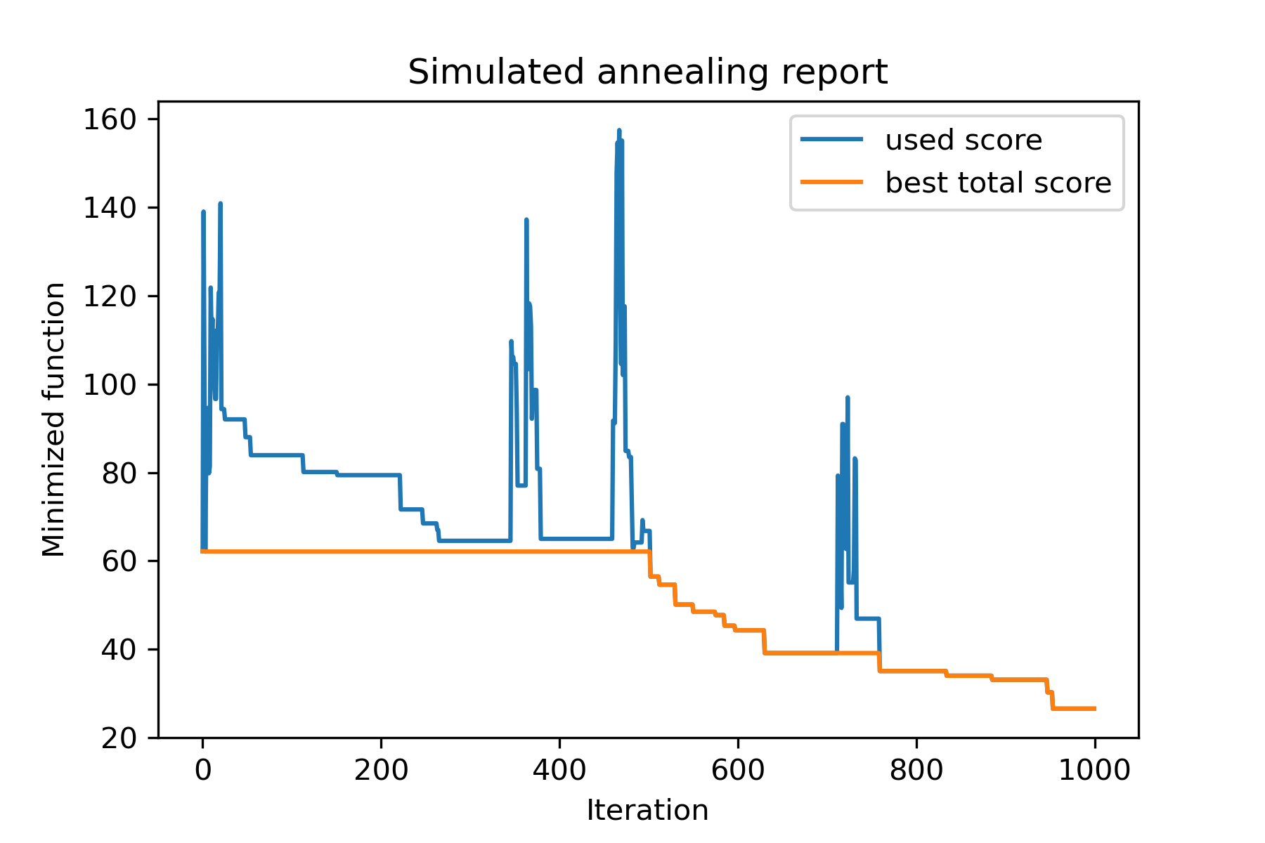
วิธีหลักของแพ็คเกจคือ run() ลองตรวจสอบว่ามันเป็นข้อโต้แย้ง:
 model . run ( start_solution ,
          mutation ,
          cooling ,
          start_temperature ,
          max_function_evals = 1000 ,
          max_iterations_without_progress = 250 ,
          step_for_reinit_temperature = 90 ,
          reinit_from_best = False ,
          seed = None )
ที่ไหน:
start_solution : อาร์เรย์ numpy; วิธีแก้ปัญหาที่ควรเริ่มต้น
mutation : ฟังก์ชั่น (อาร์เรย์, อาร์เรย์/หมายเลข) ทำหน้าที่เหมือน
 def mut ( x_as_array , temperature_as_array_or_one_number ):
    # some code
    return new_x_as_array
ฟังก์ชั่นนี้จะสร้างโซลูชันใหม่จากที่มีอยู่ ดูด้วย
cooling ระบายความร้อน: รายการฟังก์ชั่น / ฟังก์ชั่นการระบายความร้อน ฟังก์ชั่นการระบายความร้อนหรือรายการของ ดู
start_temperature : หมายเลขหรืออาร์เรย์หมายเลข (รายการ/tuple) เริ่มอุณหภูมิ สามารถเป็นหมายเลขหนึ่งหรืออาร์เรย์ของตัวเลข
max_function_evals : int, ไม่บังคับ จำนวนสูงสุดของการประเมินฟังก์ชั่น ค่าเริ่มต้นคือ 1,000
max_iterations_without_progress : int, เป็นทางเลือก จำนวนการวนซ้ำสูงสุดโดยไม่มีความคืบหน้าทั่วโลก ค่าเริ่มต้นคือ 250
step_for_reinit_temperature : int, เป็นทางเลือก หลังจากการวนซ้ำจำนวนนี้โดยไม่มีอุณหภูมิความคืบหน้าจะเริ่มต้นเช่นเดียวกับการเริ่มต้น ค่าเริ่มต้นคือ 90
reinit_from_best : บูลีนไม่บังคับ เริ่มอัลกอริทึมจากการแก้ปัญหาที่ดีที่สุดหลังจากอุณหภูมิเริ่มต้นใหม่ (หรือจากการแก้ปัญหาปัจจุบันล่าสุด) ค่าเริ่มต้นเป็นเท็จ
seed : int/none เป็นทางเลือก สุ่มเมล็ด (ถ้าจำเป็น)
ส่วนสำคัญของอัลกอริทึมคือ ฟังก์ชั่นการระบายความร้อน ฟังก์ชั่นนี้ควบคุมค่าอุณหภูมิขึ้นอยู่กับจำนวนการวนซ้ำปัจจุบันอุณหภูมิปัจจุบันและอุณหภูมิเริ่มต้น คุณสามารถสร้างฟังก์ชั่นการระบายความร้อนของคุณเองโดยใช้รูปแบบ:
 def func ( T_last , T0 , k ):
    # some code
    return T_new
ที่นี่ T_last (int/float) คือค่าอุณหภูมิจากการวนซ้ำก่อนหน้านี้ T0 (int/float) คืออุณหภูมิเริ่มต้นและ k (int> 0) คือจำนวนการวนซ้ำ คุณควรใช้ข้อมูลนี้เพื่อสร้างอุณหภูมิใหม่ T_new
ขอแนะนำให้สร้างฟังก์ชั่นของคุณเพื่อสร้างอุณหภูมิบวกเท่านั้น
ในคลาส Cooling มีฟังก์ชั่นการระบายความร้อนหลายอย่าง:
Cooling.linear(mu, Tmin = 0.01)Cooling.exponential(alpha = 0.9)Cooling.reverse(beta = 0.0005)Cooling.logarithmic(c, d = 1) - ไม่แนะนำCooling.linear_reverse() คุณสามารถเห็นพฤติกรรมของฟังก์ชั่นการระบายความร้อนโดยใช้วิธี SimulatedAnnealing.plot_temperature มาดูตัวอย่างหลายตัวอย่าง:
 from SimplestSimulatedAnnleaning import SimulatedAnnealing , Cooling


# simplest way to set cooling regime
temperature = 100
cooling = Cooling . reverse ( beta = 0.001 )
# we can temperature behaviour using this code
SimulatedAnnealing . plot_temperature ( cooling , temperature , iterations = 100 , save_as = 'reverse.png' )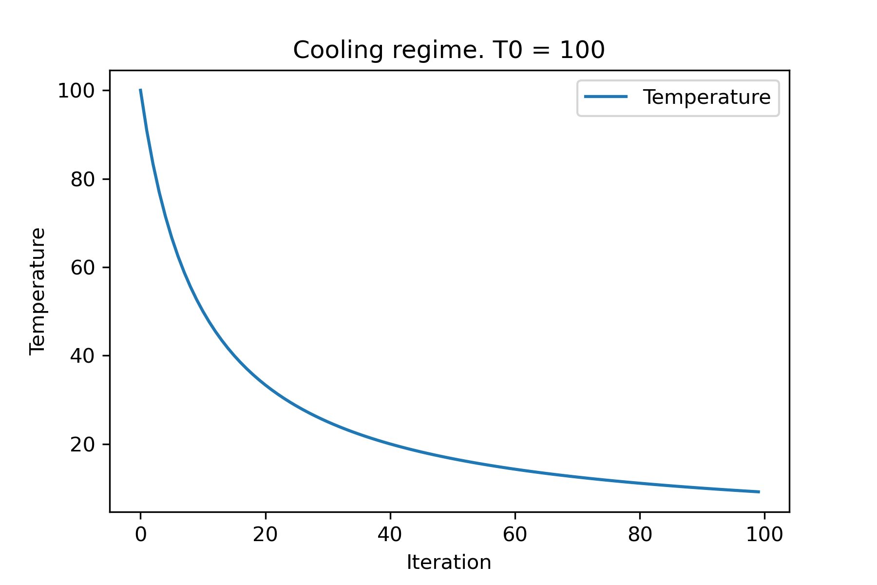
 # we can set several temparatures (for each dimention)
temperature = [ 150 , 100 , 50 ]
SimulatedAnnealing . plot_temperature ( cooling , temperature , iterations = 100 , save_as = 'reverse_diff_temp.png' )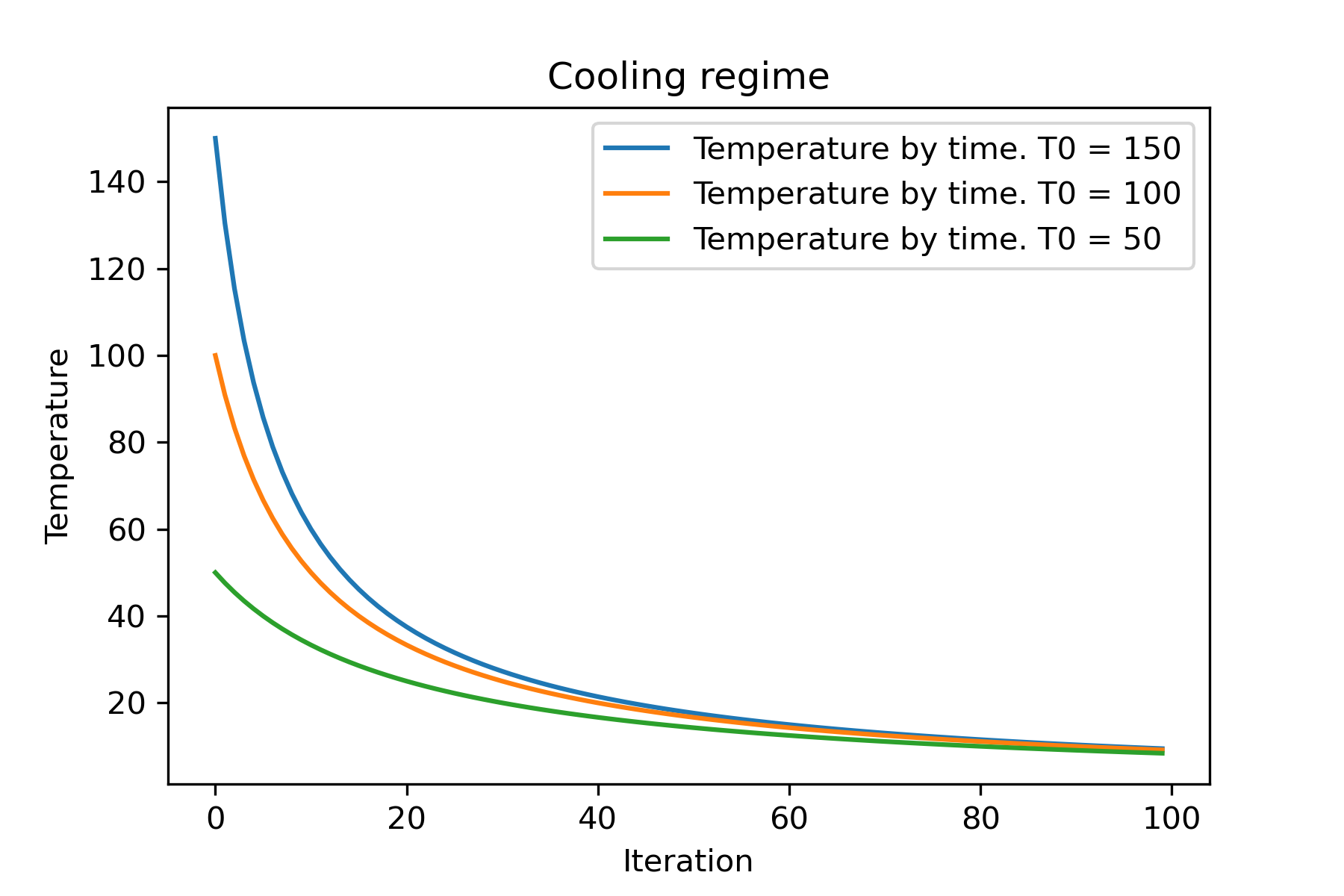
 # or several coolings (for each dimention)
temperature = 100
cooling = [
    Cooling . reverse ( beta = 0.0001 ),
    Cooling . reverse ( beta = 0.0005 ),
    Cooling . reverse ( beta = 0.001 )
    ]
SimulatedAnnealing . plot_temperature ( cooling , temperature , iterations = 100 , save_as = 'reverse_diff_beta.png' )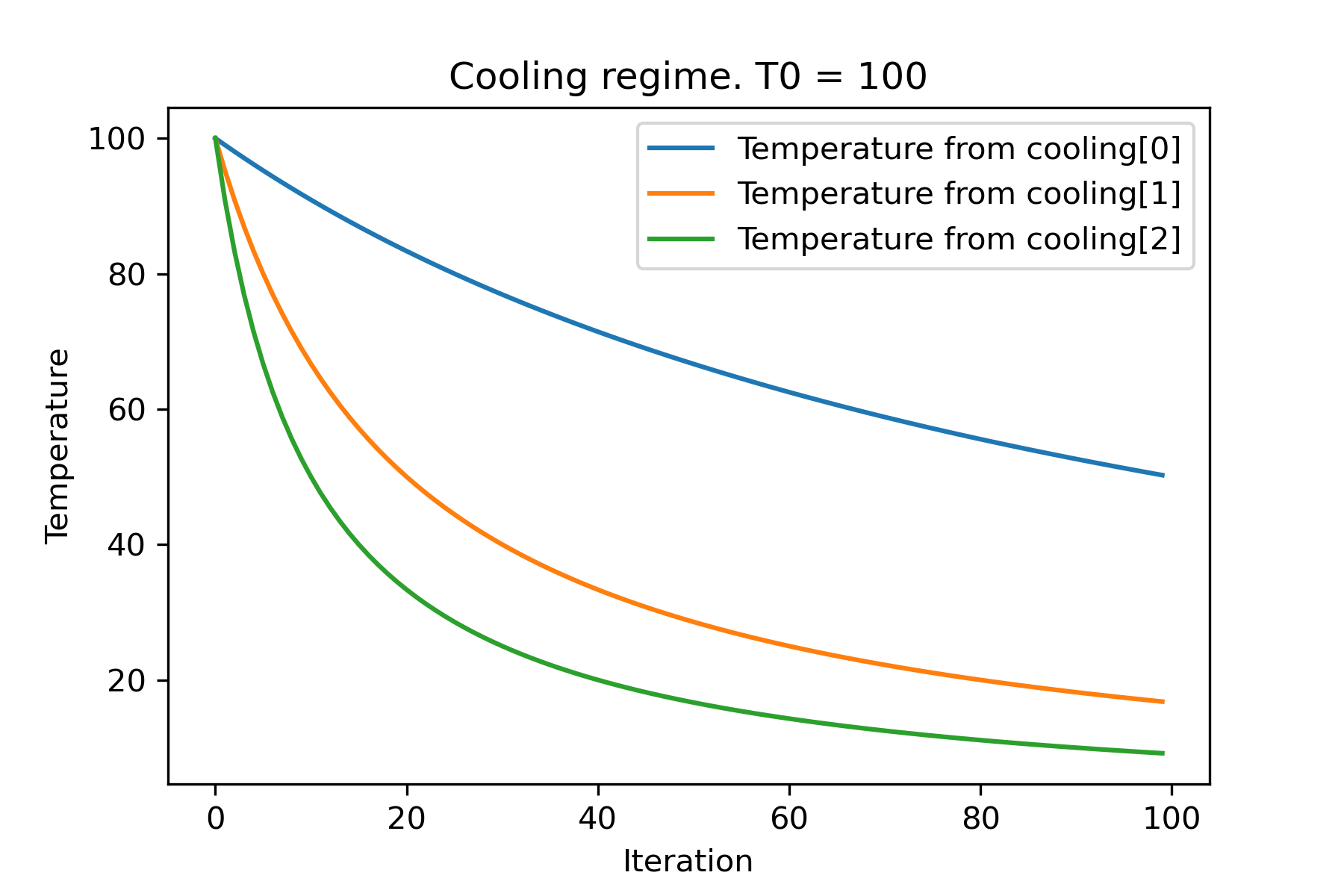
 # all supported coolling regimes

temperature = 100
cooling = [
    Cooling . linear ( mu = 1 ),
    Cooling . reverse ( beta = 0.0007 ),
    Cooling . exponential ( alpha = 0.85 ),
    Cooling . linear_reverse (),
    Cooling . logarithmic ( c = 100 , d = 1 )
    ]
SimulatedAnnealing . plot_temperature ( cooling , temperature , iterations = 100 , save_as = 'diff_temp.png' )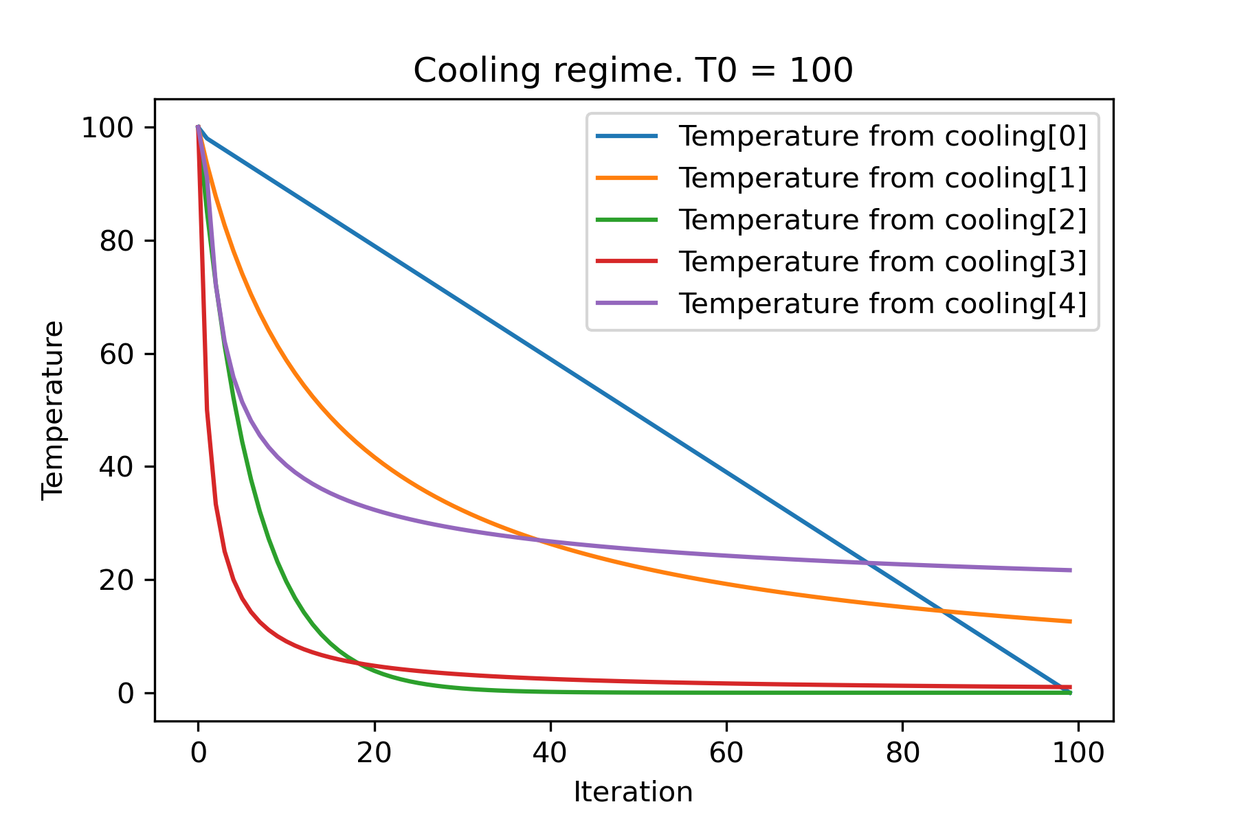
 # and we can set own temperature and cooling for each dimention!

temperature = [ 100 , 125 , 150 ]
cooling = [
    Cooling . exponential ( alpha = 0.85 ),
    Cooling . exponential ( alpha = 0.9 ),
    Cooling . exponential ( alpha = 0.95 ),
    ]
SimulatedAnnealing . plot_temperature ( cooling , temperature , iterations = 100 , save_as = 'diff_temp_and_cool.png' )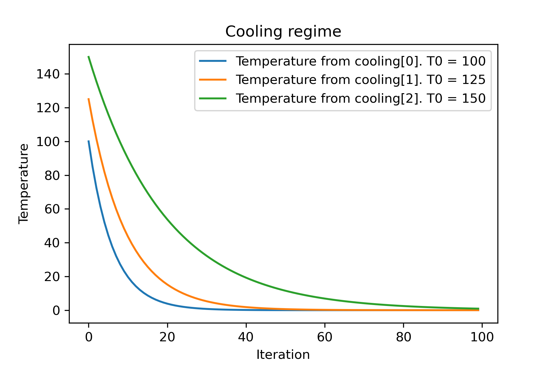
ทำไมถึงมีระบบระบายความร้อนมากมาย? สำหรับงานบางอย่างหนึ่งในนั้นสามารถดีขึ้นได้! ในสคริปต์นี้เราสามารถทดสอบการระบายความร้อนที่แตกต่างกันสำหรับฟังก์ชั่นความจริง:
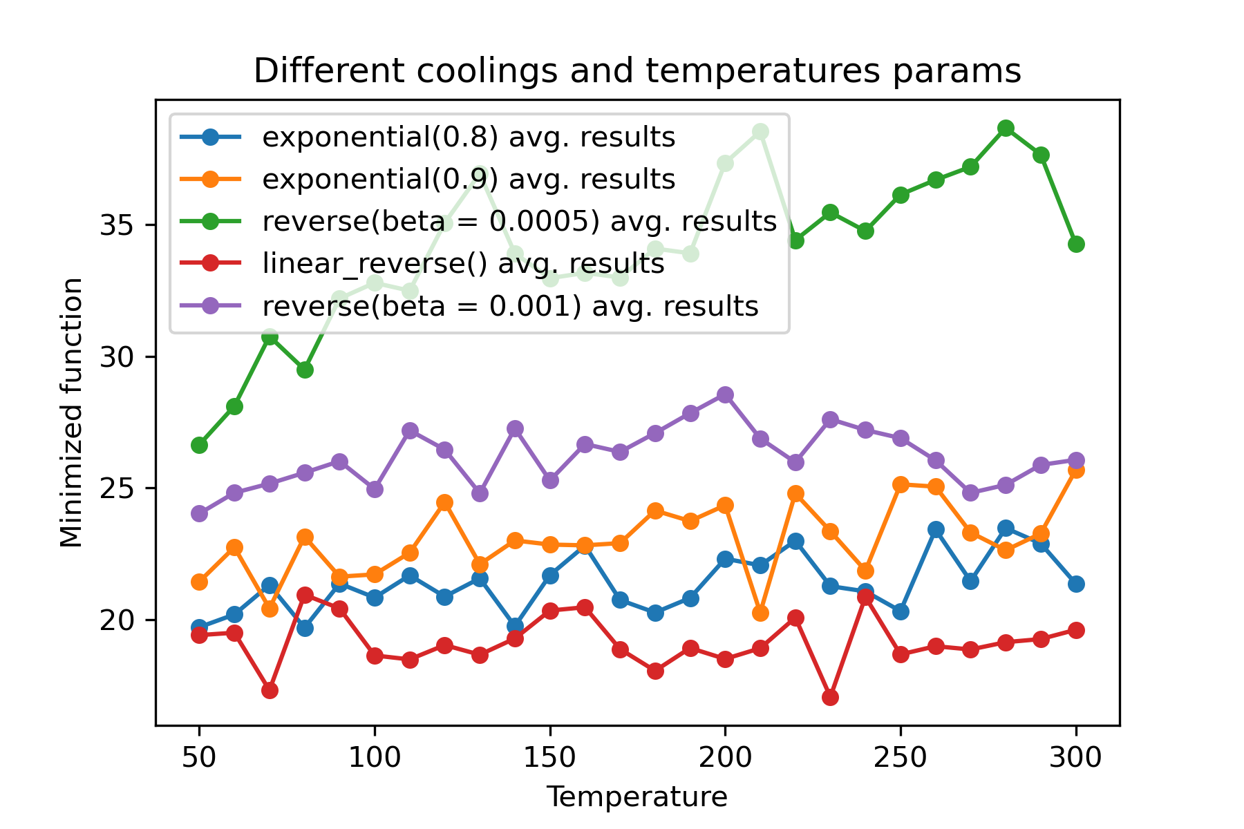
มันเป็นคุณสมบัติที่ยอดเยี่ยมใน การใช้การระบายความร้อนที่แตกต่างกันและเริ่มอุณหภูมิสำหรับแต่ละมิติ :
 import math
import numpy as np

from SimplestSimulatedAnnleaning import SimulatedAnnealing , Cooling , simple_continual_mutation


def Rastrigin ( arr ):
    return 10 * arr . size + np . sum ( arr ** 2 ) - 10 * np . sum ( np . cos ( 2 * math . pi * arr ))

dim = 5


model = SimulatedAnnealing ( Rastrigin , dim )

best_solution , best_val = model . run (
    start_solution = np . random . uniform ( - 5 , 5 , dim ),
    mutation = simple_continual_mutation ( std = 1 ),
    cooling = [ # different cooling for each dimention
        Cooling . exponential ( 0.8 ),
        Cooling . exponential ( 0.9 ),
        Cooling . reverse ( beta = 0.0005 ),
        Cooling . linear_reverse (),
        Cooling . reverse ( beta = 0.001 )
        ],
    start_temperature = 100 ,
    max_function_evals = 1000 ,
    max_iterations_without_progress = 250 ,
    step_for_reinit_temperature = 90 ,
    reinit_from_best = False
    )

print ( best_val )

model . plot_report ( save_as = 'different_coolings.png' )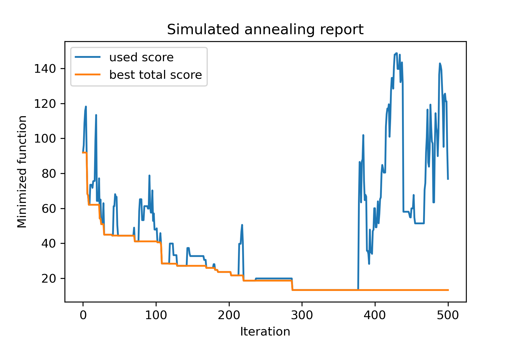
เหตุผลหลักในการใช้การระบายความร้อนหลายอย่างคือพฤติกรรมที่ระบุของแต่ละมิติ ตัวอย่างเช่นมิติแรกของพื้นที่อาจกว้างกว่ามิติที่สองมากดังนั้นจึงเป็นการดีกว่าที่จะใช้การค้นหาที่กว้างขึ้นสำหรับมิติแรก คุณสามารถผลิตได้โดยใช้ฟังก์ชั่น mut พิเศษโดยใช้ start temperatures ที่แตกต่างกันและใช้ coolings ที่แตกต่างกัน
อีกเหตุผลหนึ่งที่ใช้การระบายความร้อนหลายอย่างคือวิธีการเลือก: สำหรับ การเลือกการเย็นหลายครั้งระหว่างการแก้ปัญหาที่ดีและไม่ดีใช้ในแต่ละมิติ ดังนั้นจึงเพิ่มโอกาสในการหาทางออกที่ดีกว่า
ฟังก์ชั่นการกลายพันธุ์เป็นพารามิเตอร์ที่สำคัญที่สุด มันกำหนดพฤติกรรมของการสร้างวัตถุใหม่โดยใช้ข้อมูลเกี่ยวกับวัตถุปัจจุบันและอุณหภูมิ ฉันแนะนำให้นับหลักการเหล่านี้เมื่อสร้างฟังก์ชั่น mut :
ลองระลึกถึงโครงสร้างของ mut :
 def mut ( x_as_array , temperature_as_array_or_one_number ):
    # some code
    return new_x_as_array
ที่นี่ x_as_array เป็นวิธีแก้ปัญหาปัจจุบันและ new_x_as_array เป็นวิธีการกลายพันธุ์ (สุ่มและมีสลัวเหมือนกันตามที่คุณจำได้) นอกจากนี้คุณควรจำไว้ว่า temperature_as_array_or_one_number เป็น หมายเลข เฉพาะสำหรับการแก้ปัญหาที่ไม่ใช่หลาย multicooling มิฉะนั้น (เมื่อใช้อุณหภูมิเริ่มต้นหลายครั้งของการเย็นหรือทั้งสองอย่าง) มันเป็น อาร์เรย์ numpy ดูตัวอย่าง
ในตัวอย่างนี้ฉันแสดงวิธีเลือกวัตถุ k จาก Set with n Object ซึ่งจะลดฟังก์ชั่นบางอย่างให้น้อยที่สุด (ในตัวอย่างนี้: ค่าสัมบูรณ์ของค่ามัธยฐาน):
 import numpy as np
from SimplestSimulatedAnnleaning import SimulatedAnnealing , Cooling

SEED = 3

np . random . seed ( SEED )

Set = np . random . uniform ( low = - 15 , high = 5 , size = 100 ) # all set

dim = 10 # how many objects should we choose

indexes = np . arange ( Set . size )
# minimized function -- subset with best |median|
def min_func ( arr ):
    return abs ( np . median ( Set [ indexes [ arr . astype ( bool )]]))

# zero vectors with 'dim' ones at random positions
start_solution = np . zeros ( Set . size )
start_solution [ np . random . choice ( indexes , dim , replace = False )] = 1

# mutation function
# temperature is the number cuz we will use only 1 cooling, but it's not necessary to use it)
def mut ( x_as_array , temperature_as_array_or_one_number ):
    mask_one = x_as_array == 1
    mask_zero = np . logical_not ( mask_one )

    new_x_as_array = x_as_array . copy ()
    # replace some zeros with ones
    new_x_as_array [ np . random . choice ( indexes [ mask_one ], 1 , replace = False )] = 0
    new_x_as_array [ np . random . choice ( indexes [ mask_zero ], 1 , replace = False )] = 1

    return new_x_as_array

# creating a model
model = SimulatedAnnealing ( min_func , dim )

# run search
best_solution , best_val = model . run (
    start_solution = start_solution ,
    mutation = mut ,
    cooling = Cooling . exponential ( 0.9 ),
    start_temperature = 100 ,
    max_function_evals = 1000 ,
    max_iterations_without_progress = 100 ,
    step_for_reinit_temperature = 80 ,
    seed = SEED
    )

model . plot_report ( save_as = 'best_subset.png' )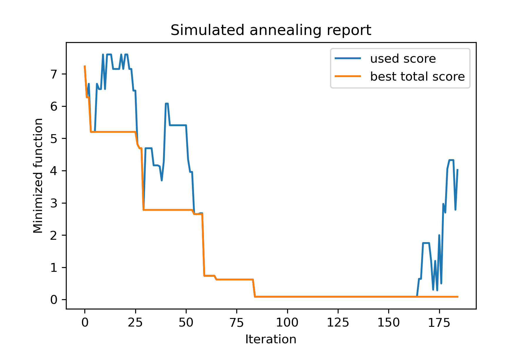
มาดูงานนี้กันเถอะ:
 split set of values {v1, v2, v3, ..., vn} to sets 0, 1, 2, 3
with their sizes (volumes determined by user) to complete best sets metric
วิธีหนึ่งในการแก้ปัญหา:
 from collections import defaultdict
import numpy as np

from SimplestSimulatedAnnleaning import SimulatedAnnealing , Cooling

################### useful methods

def counts_to_vec ( dic_count ):
    """
    converts dictionary like {1: 3, 2: 4}
    to array [1, 1, 1, 2, 2, 2, 2]
    """
    arrs = [ np . full ( val , fill_value = key ) for key , val in dic_count . items ()]

    return np . concatenate ( tuple ( arrs ))

def vec_to_indexes_dict ( vector ):
    """
    converts vector like [1, 0, 1, 2, 2]
    to dictionary with indexes {1: [0, 2], 2: [3, 4]}
    """

    res = defaultdict ( list )

    for i , v in enumerate ( vector ):
        res [ v ]. append ( i )

    return { int ( key ): np . array ( val ) for key , val in res . items () if key != 0 }


#################### START PARAMS

SEED = 3

np . random . seed ( SEED )

Set = np . random . uniform ( low = - 15 , high = 5 , size = 100 ) # all set
Set_indexes = np . arange ( Set . size )

# how many objects should be in each set
dim_dict = {
    1 : 10 ,
    2 : 10 ,
    3 : 7 ,
    4 : 14
}


# minimized function: sum of means vy each split set
def min_func ( arr ):

    indexes_dict = vec_to_indexes_dict ( arr )

    means = [ np . mean ( Set [ val ]) for val in indexes_dict . values ()]

    return sum ( means )

# zero vector with available set labels at random positions
start_solution = np . zeros ( Set . size , dtype = np . int8 )
labels_vec = counts_to_vec ( dim_dict )
start_solution [ np . random . choice ( Set_indexes , labels_vec . size , replace = False )] = labels_vec


def choice ( count = 3 ):
    return np . random . choice ( Set_indexes , count , replace = False )

# mutation function
# temperature is the number cuz we will use only 1 cooling, but it's not necessary to use it)
def mut ( x_as_array , temperature_as_array_or_one_number ):

    new_x_as_array = x_as_array . copy ()
    # replace some values

    while True :
        inds = choice ()

        if np . unique ( new_x_as_array [ inds ]). size == 1 : # there is no sense to replace same values
            continue
        new_x_as_array [ inds ] = new_x_as_array [ np . random . permutation ( inds )]

        return new_x_as_array

# creating a model
model = SimulatedAnnealing ( min_func , Set_indexes . size )

# run search
best_solution , best_val = model . run (
    start_solution = start_solution ,
    mutation = mut ,
    cooling = Cooling . exponential ( 0.9 ),
    start_temperature = 100 ,
    max_function_evals = 1000 ,
    max_iterations_without_progress = 100 ,
    step_for_reinit_temperature = 80 ,
    seed = SEED ,
    reinit_from_best = True
    )

model . plot_report ( save_as = 'best_split.png' )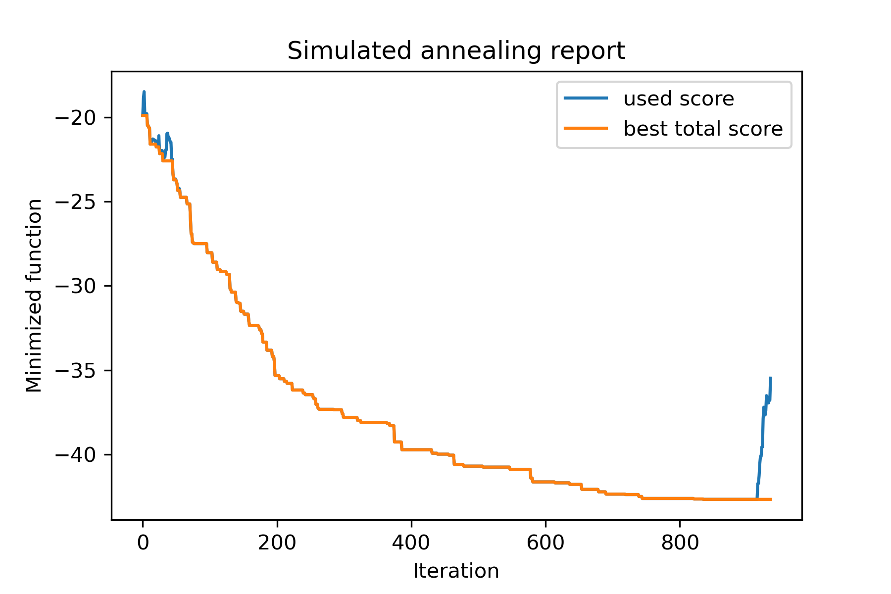
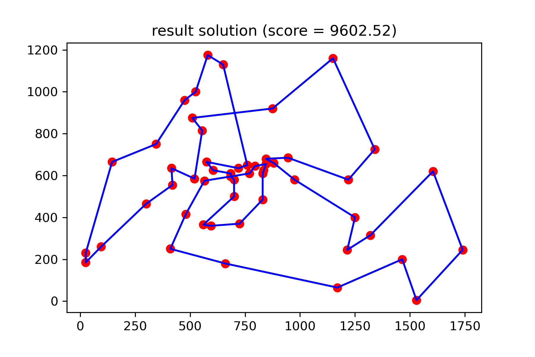
มาลองแก้ปัญหาพนักงานขายการเดินทางสำหรับงาน Berlin52 ในงานนี้มี 52 เมืองที่มีพิกัดจากไฟล์
ประการแรกลองนำเข้าแพ็คเกจ:
 import math
import numpy as np
import pandas as pd
import matplotlib . pyplot as plt

from SimplestSimulatedAnnleaning import SimulatedAnnealing , Cooling
ตั้งค่าเมล็ดพันธุ์สำหรับการทำซ้ำ:
 SEED = 1
np . random . seed ( SEED )
อ่านพิกัดและสร้างเมทริกซ์ระยะทาง:
 # read coordinates
coords = pd . read_csv ( 'berlin52_coords.txt' , sep = ' ' , header = None , names = [ 'index' , 'x' , 'y' ])

# dim is equal to count of cities
dim = coords . shape [ 0 ]

# distance matrix
distances = np . empty (( dim , dim ))

for i in range ( dim ):
    distances [ i , i ] = 0
    for j in range ( i + 1 , dim ):
        d = math . sqrt ( np . sum (( coords . iloc [ i , 1 :] - coords . iloc [ j , 1 :]) ** 2 ))
        distances [ i , j ] = d
        distances [ j , i ] = d
สร้างโซลูชันการเริ่มต้นแบบสุ่ม:
 indexes = np . arange ( dim )
# some start solution (indexes shuffle)
start_solution = np . random . choice ( indexes , dim , replace = False )
กำหนดฟังก์ชั่นที่คำนวณความยาวของวิธี:
 # minized function
def way_length ( arr ):
    s = 0
    for i in range ( 1 , dim ):
        s += distances [ arr [ i - 1 ], arr [ i ]]
    # also we should end the way in the beggining
    s += distances [ arr [ - 1 ], arr [ 1 ]]

    return s
ลองมองเห็นการแก้ปัญหาเริ่มต้นกันเถอะ:
 def plotData ( indices , title , save_as = None ):

    # create a list of the corresponding city locations:
    locs = [ coords . iloc [ i , 1 :] for i in indices ]
    locs . append ( coords . iloc [ indices [ 0 ], 1 :])

    # plot a line between each pair of consequtive cities:
    plt . plot ( * zip ( * locs ), linestyle = '-' , color = 'blue' )

    # plot the dots representing the cities:
    plt . scatter ( coords . iloc [:, 1 ], coords . iloc [:, 2 ], marker = 'o' , s = 40 , color = 'red' )
    plt . title ( title )

    if not ( save_as is None ):  plt . savefig ( save_as , dpi = 300 )

    plt . show ()


# let's plot start solution
plotData ( start_solution , f'start random solution (score = { round ( way_length ( start_solution ), 2 ) } )' , 'salesman_start.png' )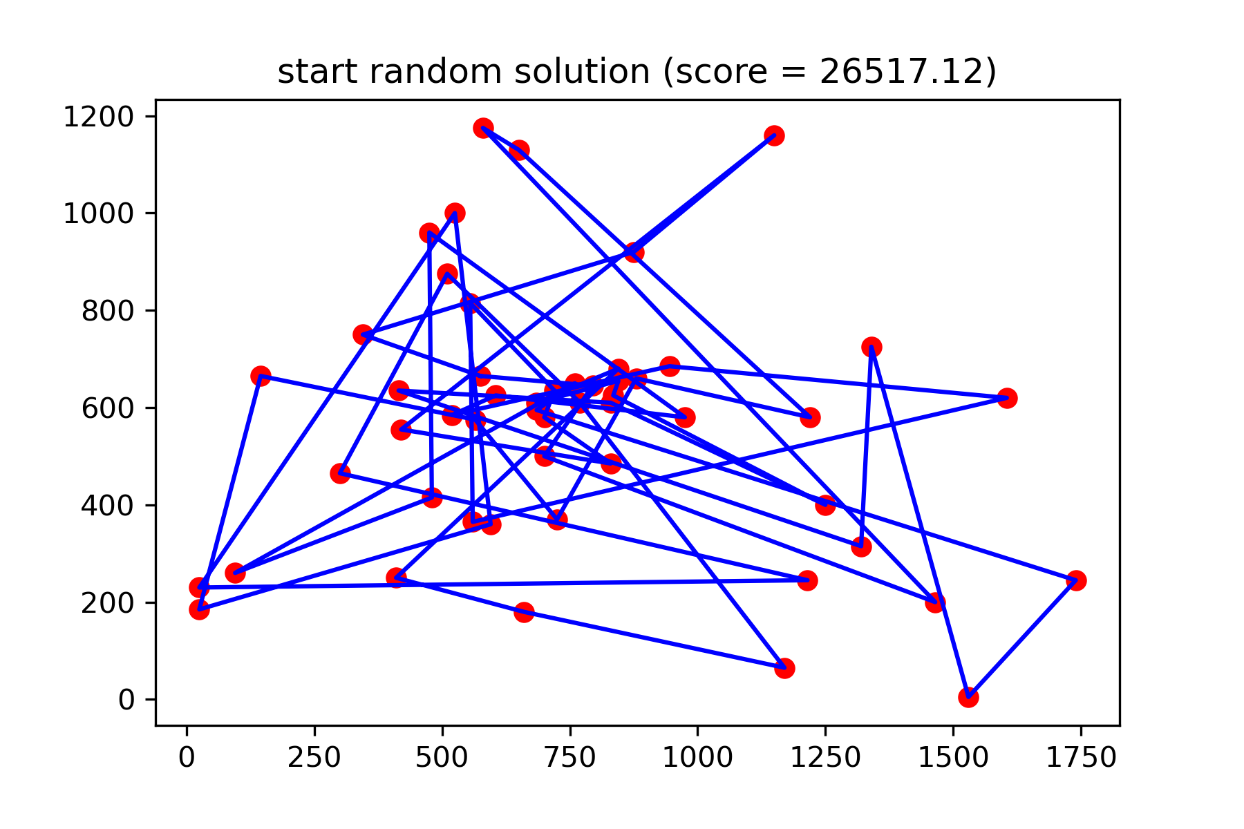
มันไม่ใช่ทางออกที่ดีจริงๆ ฉันต้องการสร้างฟังก์ชั่นการกลายพันธุ์นี้สำหรับงานนี้:
 def mut ( x_as_array , temperature_as_array_or_one_number ):
    # random indexes
    rand_inds = np . random . choice ( indexes , 3 , replace = False )
    # shuffled indexes
    goes_to = np . random . permutation ( rand_inds )

    # just replace some positions in the array
    new_x_as_array = x_as_array . copy ()
    new_x_as_array [ rand_inds ] = new_x_as_array [ goes_to ]

    return new_x_as_array
เริ่มค้นหา:
 # creating a model
model = SimulatedAnnealing ( way_length , dim )

# run search
best_solution , best_val = model . run (
    start_solution = start_solution ,
    mutation = mut ,
    cooling = Cooling . exponential ( 0.9 ),
    start_temperature = 100 ,
    max_function_evals = 15000 ,
    max_iterations_without_progress = 2000 ,
    step_for_reinit_temperature = 80 ,
    reinit_from_best = True ,
    seed = SEED
    )

model . plot_report ( save_as = 'best_salesman.png' )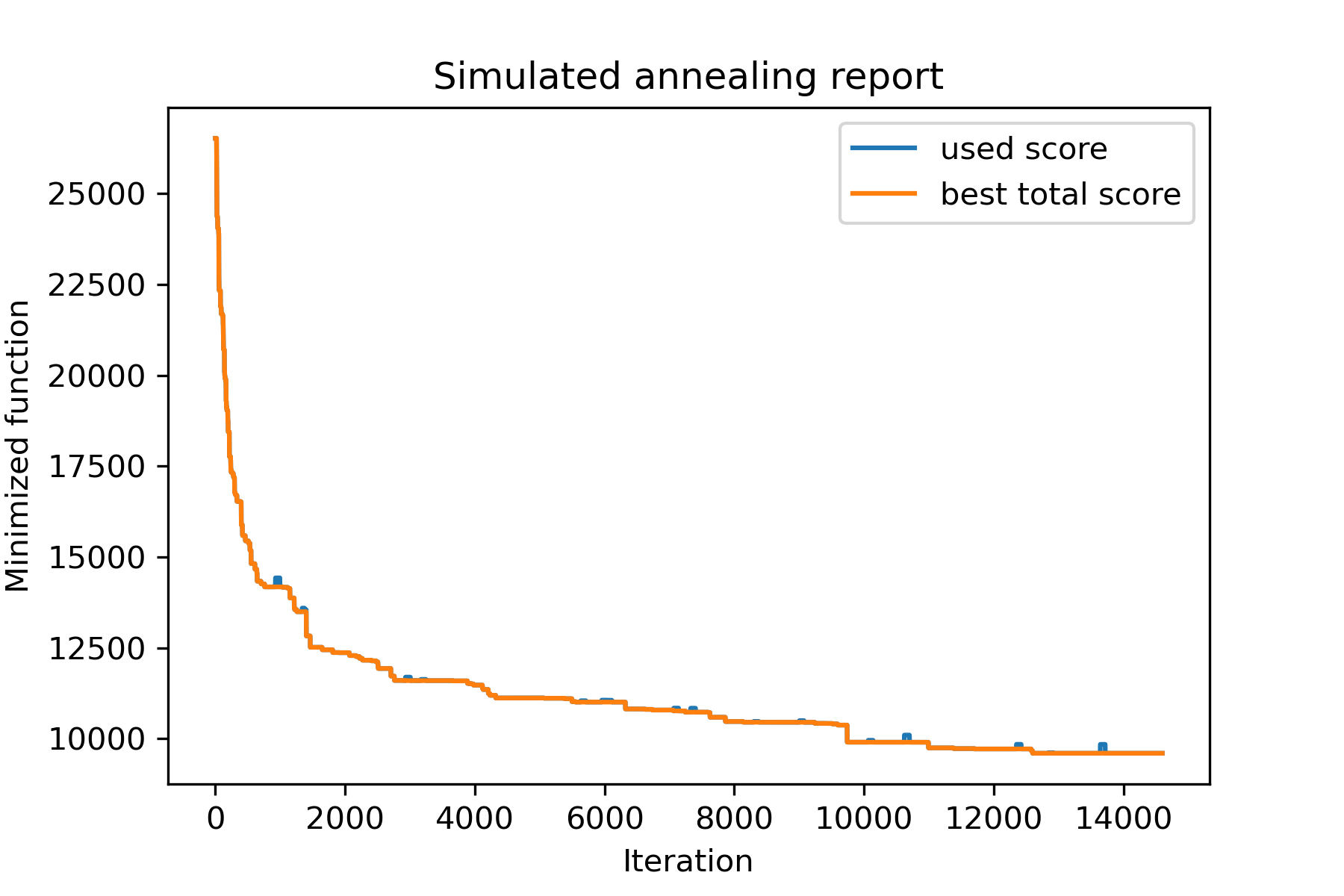
และดูทางออกที่ดีกว่าของเรา:
plotData ( best_solution , f'result solution (score = { round ( best_val , 2 ) } )' , 'salesman_result.png' )