SimplestSimulatedAnnealing
1.0.0
Einfachste Implementierung (aus DPEA) der simulierten Annealing -Methode
pip install SimplestSimulatedAnnealing
Dies ist der evolutionäre Algorithmus zur Funktionsminimierung .
Schritte:
f bestimmen, die minimiert werden mussx0 bestimmen (kann zufällig sein)mut . Diese Funktion sollte eine neue (kann zufällige) x1 -Lösung unter Verwendung von Informationen zu x0 und Temperatur T ergeben.cooling (en) (Temperaturverhalten)Tx0 Lösung und f(x0) beste Punktzahlx1 = mut(x0) und berechnen Sie f(x1)f(x1) < f(x0) , fanden wir eine bessere Lösung x0 = x1 . Andernfalls können wir x1 durch x0 durch exp((f(x0) - f(x1)) / T)T mit der cooling : T = cooling(T)Pakete importieren:
 import math
import numpy as np

from SimplestSimulatedAnnleaning import SimulatedAnnealing , Cooling , simple_continual_mutation
Minimierte Funktion bestimmen (Rastrigin):
 def Rastrigin ( arr ):
    return 10 * arr . size + np . sum ( arr ** 2 ) - 10 * np . sum ( np . cos ( 2 * math . pi * arr ))

dim = 5
Wir werden die einfachste Gauß -Mutation verwenden:
mut = simple_continual_mutation ( std = 0.5 )Modellobjekt erstellen (Funktion und Dimension festlegen):
model = SimulatedAnnealing ( Rastrigin , dim )Beginnen Sie mit der Suche und sehen Sie sich den Bericht an:
 best_solution , best_val = model . run (
    start_solution = np . random . uniform ( - 5 , 5 , dim ),
    mutation = mut ,
    cooling = Cooling . exponential ( 0.9 ),
    start_temperature = 100 ,
    max_function_evals = 1000 ,
    max_iterations_without_progress = 100 ,
    step_for_reinit_temperature = 80
    )

model . plot_report ( save_as = 'simple_example.png' )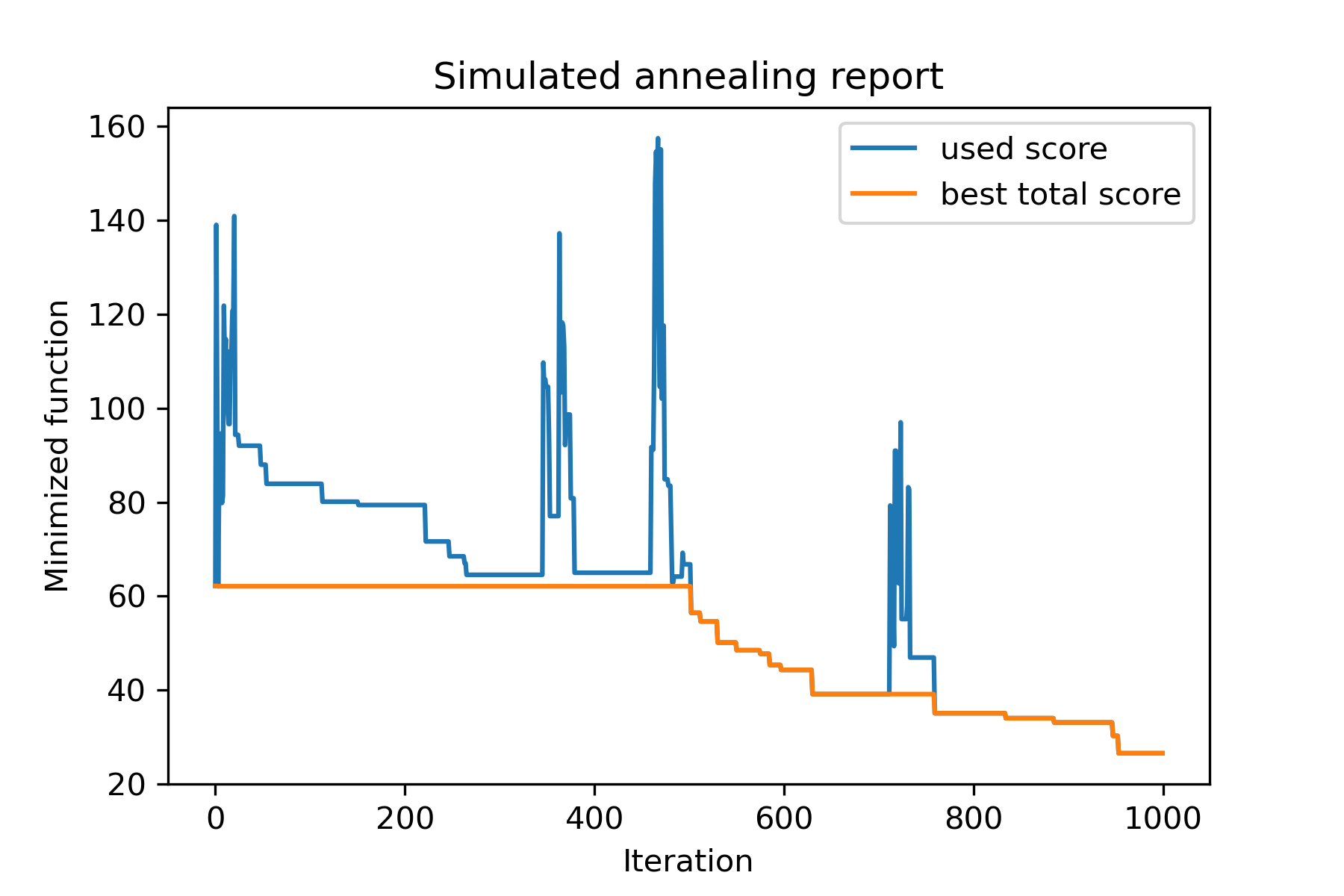
Die Hauptmethode des Pakets wird run() . Überprüfen Sie, ob es sich um Argumente handelt:
 model . run ( start_solution ,
          mutation ,
          cooling ,
          start_temperature ,
          max_function_evals = 1000 ,
          max_iterations_without_progress = 250 ,
          step_for_reinit_temperature = 90 ,
          reinit_from_best = False ,
          seed = None )
Wo:
start_solution : Numpy Array; Lösung, aus der es beginnen sollte.
mutation : Funktion (Array, Array/Nummer). Funktion wie
 def mut ( x_as_array , temperature_as_array_or_one_number ):
    # some code
    return new_x_as_array
Diese Funktion erzeugt neue Lösungen aus vorhanden. Siehe auch
cooling : Kühlfunktion / Funktionsliste. Kühlfunktion oder eine Liste von Einsen. Sehen
start_temperature : nummer oder nummernarray (list/tuple). Starttemperaturen. Kann eine Nummer oder eine Reihe von Zahlen sein.
max_function_evals : int, optional. Maximale Anzahl von Funktionsbewertungen. Der Standard ist 1000.
max_iterations_without_progress : int, optional. Maximale Anzahl von Iterationen ohne globalen Fortschritt. Der Standard ist 250.
step_for_reinit_temperature : INT, optional. Nach dieser Anzahl von Iterationen ohne Fortschritt werden die Temperaturen wie Start initialisiert. Der Standard ist 90.
reinit_from_best : Boolean, optional. Starten Sie den Algorithmus aus der besten Lösung nach den Reinitentemperaturen (oder aus der letzten Stromlösung). Der Standard ist falsch.
seed : int/none, optional. Zufälliger Samen (falls erforderlich)
Der wichtige Teil des Algorithmus ist die Kühlfunktion . Diese Funktion steuert den Temperaturwert, der von der aktuellen Iterationszahl, der Stromtemperatur und der Starttemperatur abhängt. Sie können Ihre eigene Kühlfunktion mit Muster erstellen:
 def func ( T_last , T0 , k ):
    # some code
    return T_new
Hier ist T_last (int/float) der Temperaturwert aus der vorherigen Iteration, T0 (int/float) ist die Starttemperatur und k (int> 0) ist die Anzahl der Iteration. U sollten einige dieser Informationen verwenden, um eine neue Temperatur T_new zu erstellen.
Es wird dringend empfohlen, Ihre Funktion zu erstellen, um nur positive Temperatur zu erzeugen.
In Cooling gibt es mehrere Kühlfunktionen:
Cooling.linear(mu, Tmin = 0.01)Cooling.exponential(alpha = 0.9)Cooling.reverse(beta = 0.0005)Cooling.logarithmic(c, d = 1) - nicht empfohlenCooling.linear_reverse() U kann das Verhalten der Kühlfunktion unter Verwendung von SimulatedAnnealing.plot_temperature sehen. Lassen Sie uns mehrere Beispiele sehen:
 from SimplestSimulatedAnnleaning import SimulatedAnnealing , Cooling


# simplest way to set cooling regime
temperature = 100
cooling = Cooling . reverse ( beta = 0.001 )
# we can temperature behaviour using this code
SimulatedAnnealing . plot_temperature ( cooling , temperature , iterations = 100 , save_as = 'reverse.png' )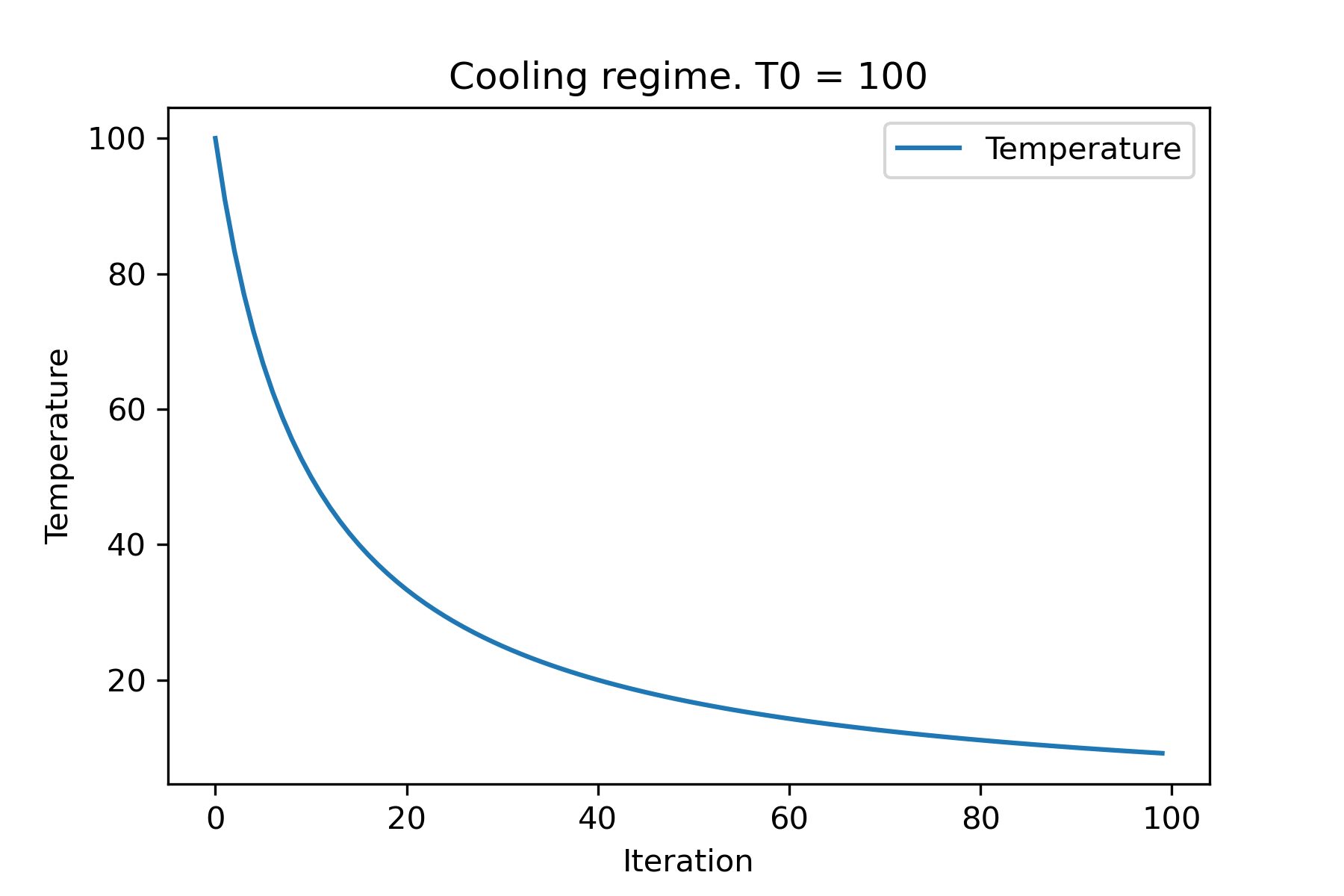
 # we can set several temparatures (for each dimention)
temperature = [ 150 , 100 , 50 ]
SimulatedAnnealing . plot_temperature ( cooling , temperature , iterations = 100 , save_as = 'reverse_diff_temp.png' )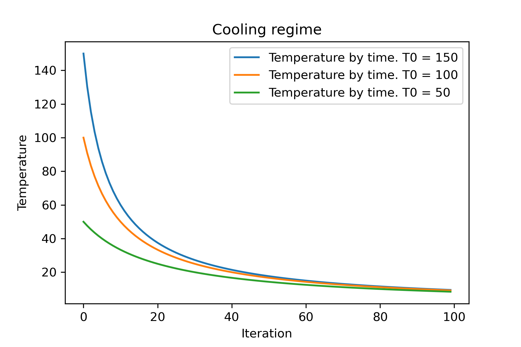
 # or several coolings (for each dimention)
temperature = 100
cooling = [
    Cooling . reverse ( beta = 0.0001 ),
    Cooling . reverse ( beta = 0.0005 ),
    Cooling . reverse ( beta = 0.001 )
    ]
SimulatedAnnealing . plot_temperature ( cooling , temperature , iterations = 100 , save_as = 'reverse_diff_beta.png' )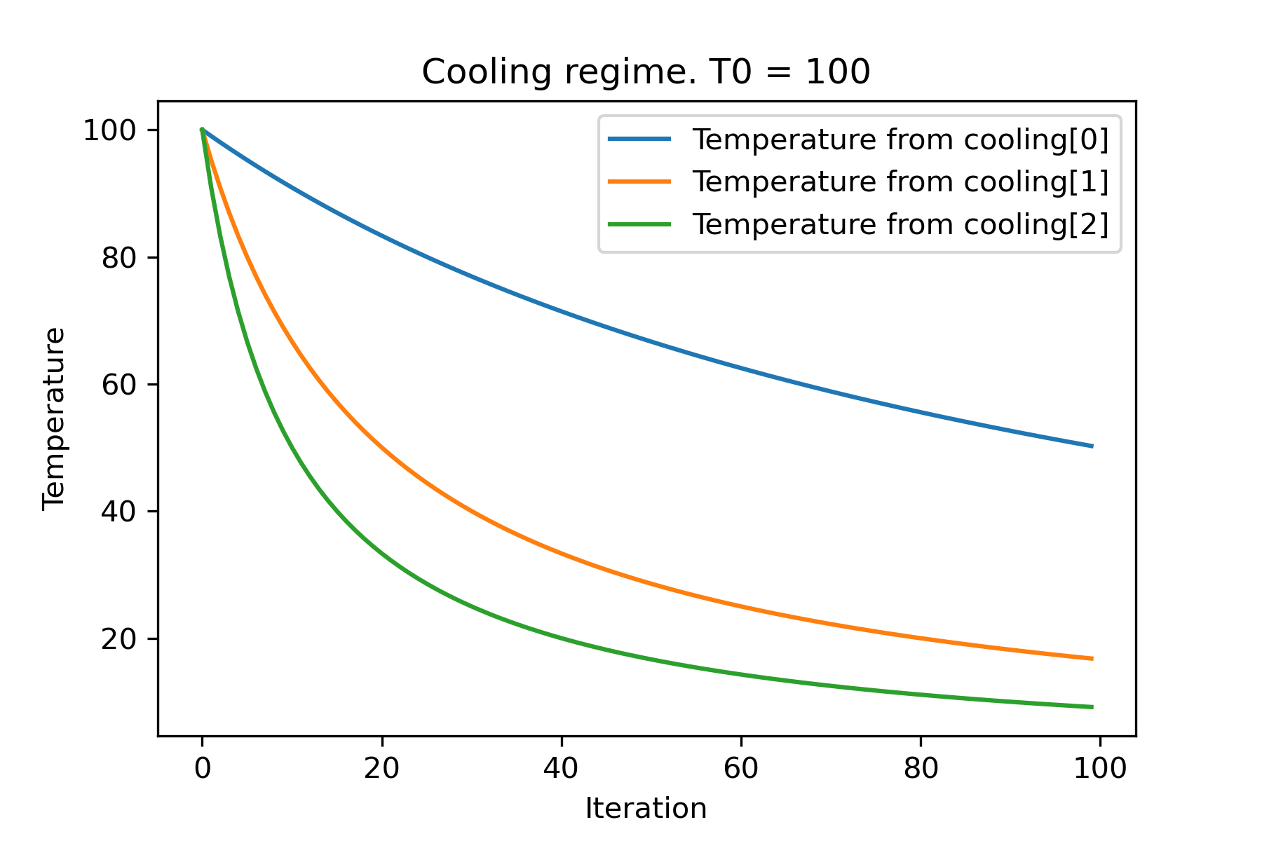
 # all supported coolling regimes

temperature = 100
cooling = [
    Cooling . linear ( mu = 1 ),
    Cooling . reverse ( beta = 0.0007 ),
    Cooling . exponential ( alpha = 0.85 ),
    Cooling . linear_reverse (),
    Cooling . logarithmic ( c = 100 , d = 1 )
    ]
SimulatedAnnealing . plot_temperature ( cooling , temperature , iterations = 100 , save_as = 'diff_temp.png' )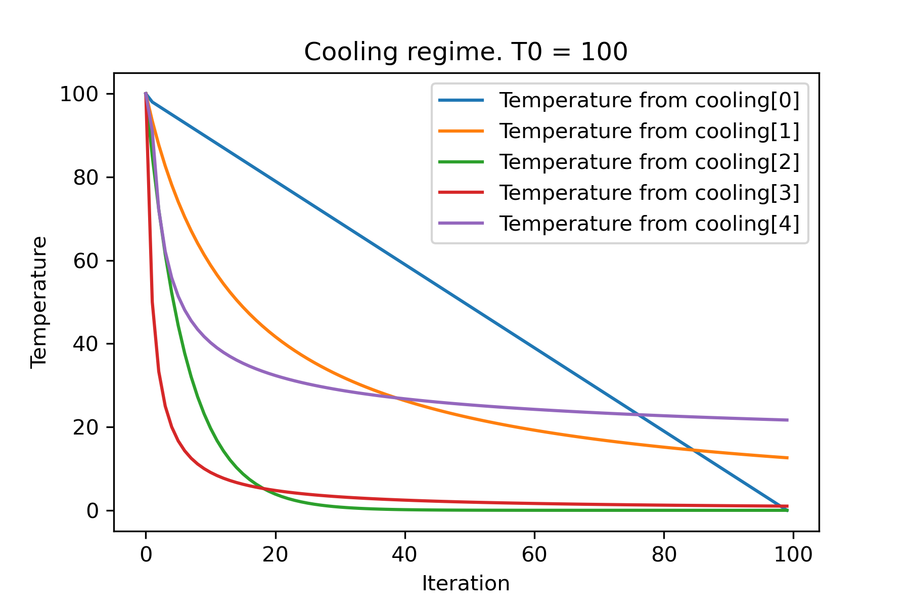
 # and we can set own temperature and cooling for each dimention!

temperature = [ 100 , 125 , 150 ]
cooling = [
    Cooling . exponential ( alpha = 0.85 ),
    Cooling . exponential ( alpha = 0.9 ),
    Cooling . exponential ( alpha = 0.95 ),
    ]
SimulatedAnnealing . plot_temperature ( cooling , temperature , iterations = 100 , save_as = 'diff_temp_and_cool.png' )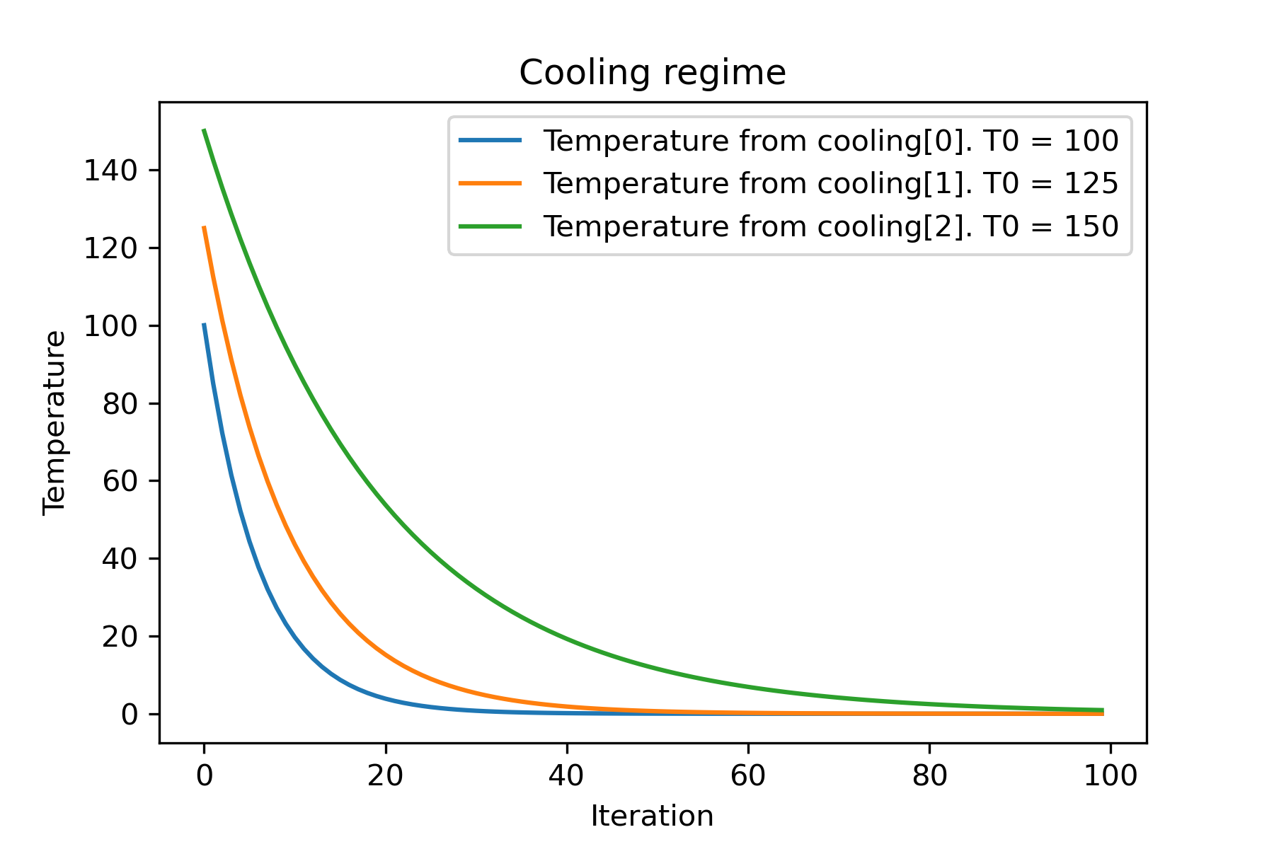
Warum gibt es so viele Kühlregime? Für eine bestimmte Aufgabe kann einer von ihnen so besser sein! In diesem Skript können wir eine andere Kühlung für die Rastring -Funktion testen:
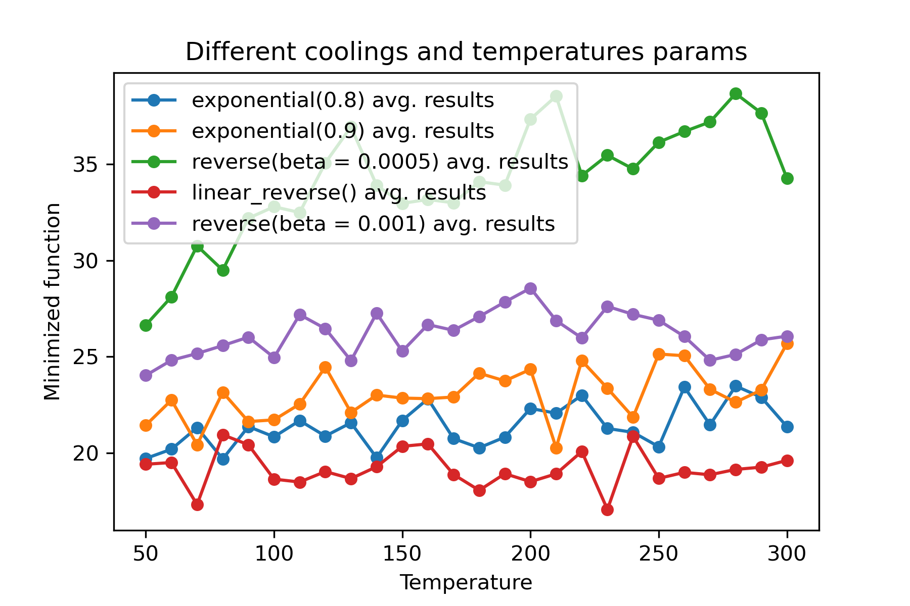
Es ist eine erstaunliche Funktion , verschiedene Kühlungen und Starttemperaturen für jede Dimension zu verwenden :
 import math
import numpy as np

from SimplestSimulatedAnnleaning import SimulatedAnnealing , Cooling , simple_continual_mutation


def Rastrigin ( arr ):
    return 10 * arr . size + np . sum ( arr ** 2 ) - 10 * np . sum ( np . cos ( 2 * math . pi * arr ))

dim = 5


model = SimulatedAnnealing ( Rastrigin , dim )

best_solution , best_val = model . run (
    start_solution = np . random . uniform ( - 5 , 5 , dim ),
    mutation = simple_continual_mutation ( std = 1 ),
    cooling = [ # different cooling for each dimention
        Cooling . exponential ( 0.8 ),
        Cooling . exponential ( 0.9 ),
        Cooling . reverse ( beta = 0.0005 ),
        Cooling . linear_reverse (),
        Cooling . reverse ( beta = 0.001 )
        ],
    start_temperature = 100 ,
    max_function_evals = 1000 ,
    max_iterations_without_progress = 250 ,
    step_for_reinit_temperature = 90 ,
    reinit_from_best = False
    )

print ( best_val )

model . plot_report ( save_as = 'different_coolings.png' )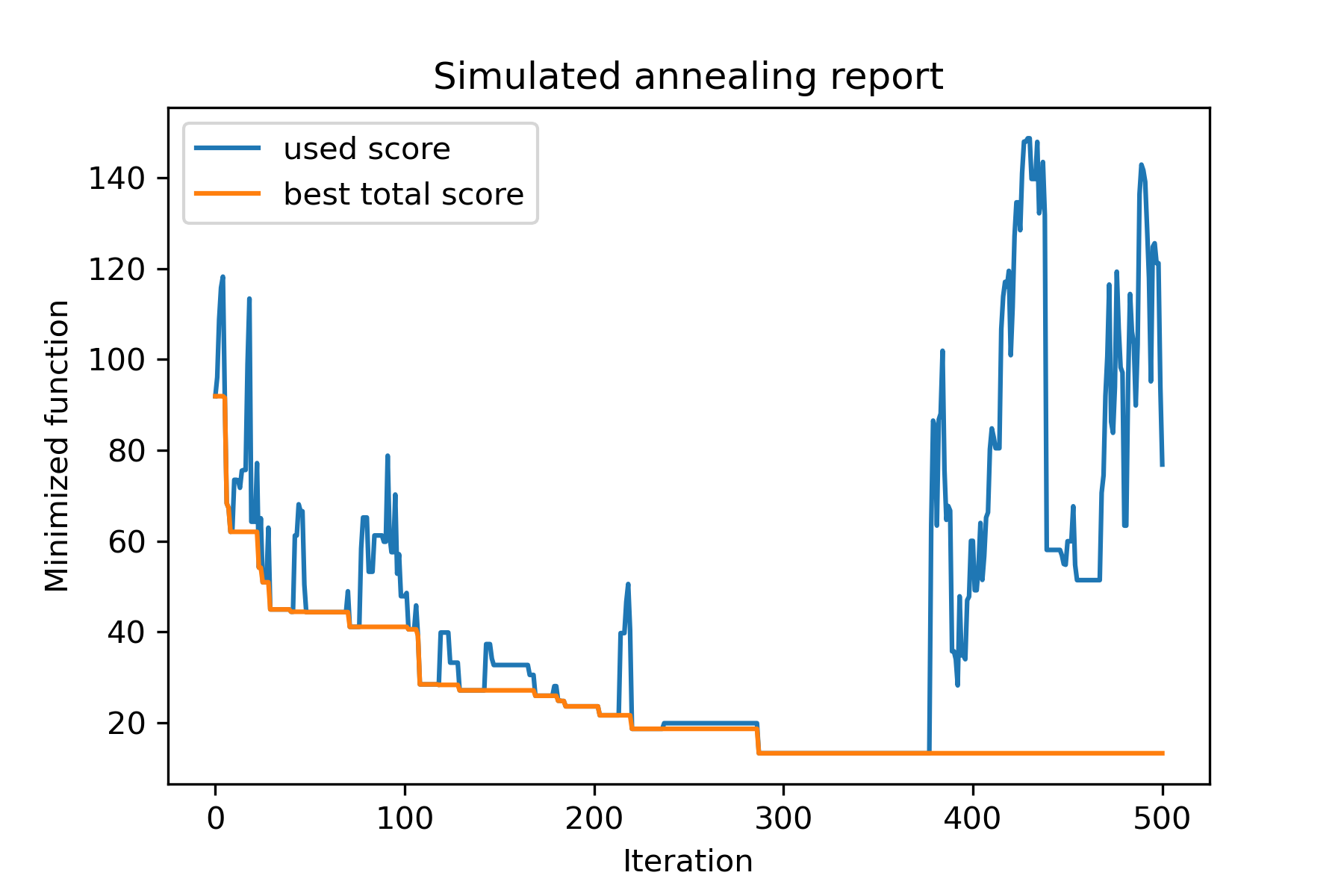
Der Hauptgrund für die Verwendung mehrerer Kühlungen ist das angebene Verhalten jeder Dimension. Zum Beispiel kann die erste Dimension des Raums viel breiter sein als die zweite Dimension, daher ist es besser, eine breitere Suche nach der ersten Dimension zu verwenden. u können es unter Verwendung einer speziellen mut -Funktion, mit unterschiedlichen start temperatures und mit unterschiedlichen coolings produzieren.
Ein weiterer Grund für die Verwendung mehrerer Kühlungen ist die Art der Auswahl: Bei mehreren Kühlungen zwischen guten und schlechten Lösungen gilt für jede Dimension . Es erhöht also die Chancen, eine bessere Lösung zu finden.
Die Mutationsfunktion ist der wichtigste Parameter. Es bestimmt das Verhalten, neue Objekte mit Informationen zu aktuellem Objekt und über die Temperatur zu erstellen. Ich empfehle, diese Prinzipien beim Erstellen von mut -Funktion zu zählen:
Erinnern wir uns an die Struktur von mut :
 def mut ( x_as_array , temperature_as_array_or_one_number ):
    # some code
    return new_x_as_array
Hier ist x_as_array die aktuelle Lösung und new_x_as_array ist die mutierte Lösung (zufällig und mit demselben Schwach, wie Sie sich erinnern). Sie sollten sich auch daran erinnern, dass temperature_as_array_or_one_number nur für Nicht-Multikooling-Lösung eine Nummer ist. Andernfalls (bei Verwendung mehrerer Starttemperaturen mehrerer Kühlungen oder beides) handelt es sich um Numpy -Array . Siehe Beispiele
In diesem Beispiel zeige ich, wie Sie k -Objekte aus NET mit n -Objekten ausgewählt haben, die eine gewisse Funktion minimieren (in diesem Beispiel: Absolutwert des Medians):
 import numpy as np
from SimplestSimulatedAnnleaning import SimulatedAnnealing , Cooling

SEED = 3

np . random . seed ( SEED )

Set = np . random . uniform ( low = - 15 , high = 5 , size = 100 ) # all set

dim = 10 # how many objects should we choose

indexes = np . arange ( Set . size )
# minimized function -- subset with best |median|
def min_func ( arr ):
    return abs ( np . median ( Set [ indexes [ arr . astype ( bool )]]))

# zero vectors with 'dim' ones at random positions
start_solution = np . zeros ( Set . size )
start_solution [ np . random . choice ( indexes , dim , replace = False )] = 1

# mutation function
# temperature is the number cuz we will use only 1 cooling, but it's not necessary to use it)
def mut ( x_as_array , temperature_as_array_or_one_number ):
    mask_one = x_as_array == 1
    mask_zero = np . logical_not ( mask_one )

    new_x_as_array = x_as_array . copy ()
    # replace some zeros with ones
    new_x_as_array [ np . random . choice ( indexes [ mask_one ], 1 , replace = False )] = 0
    new_x_as_array [ np . random . choice ( indexes [ mask_zero ], 1 , replace = False )] = 1

    return new_x_as_array

# creating a model
model = SimulatedAnnealing ( min_func , dim )

# run search
best_solution , best_val = model . run (
    start_solution = start_solution ,
    mutation = mut ,
    cooling = Cooling . exponential ( 0.9 ),
    start_temperature = 100 ,
    max_function_evals = 1000 ,
    max_iterations_without_progress = 100 ,
    step_for_reinit_temperature = 80 ,
    seed = SEED
    )

model . plot_report ( save_as = 'best_subset.png' )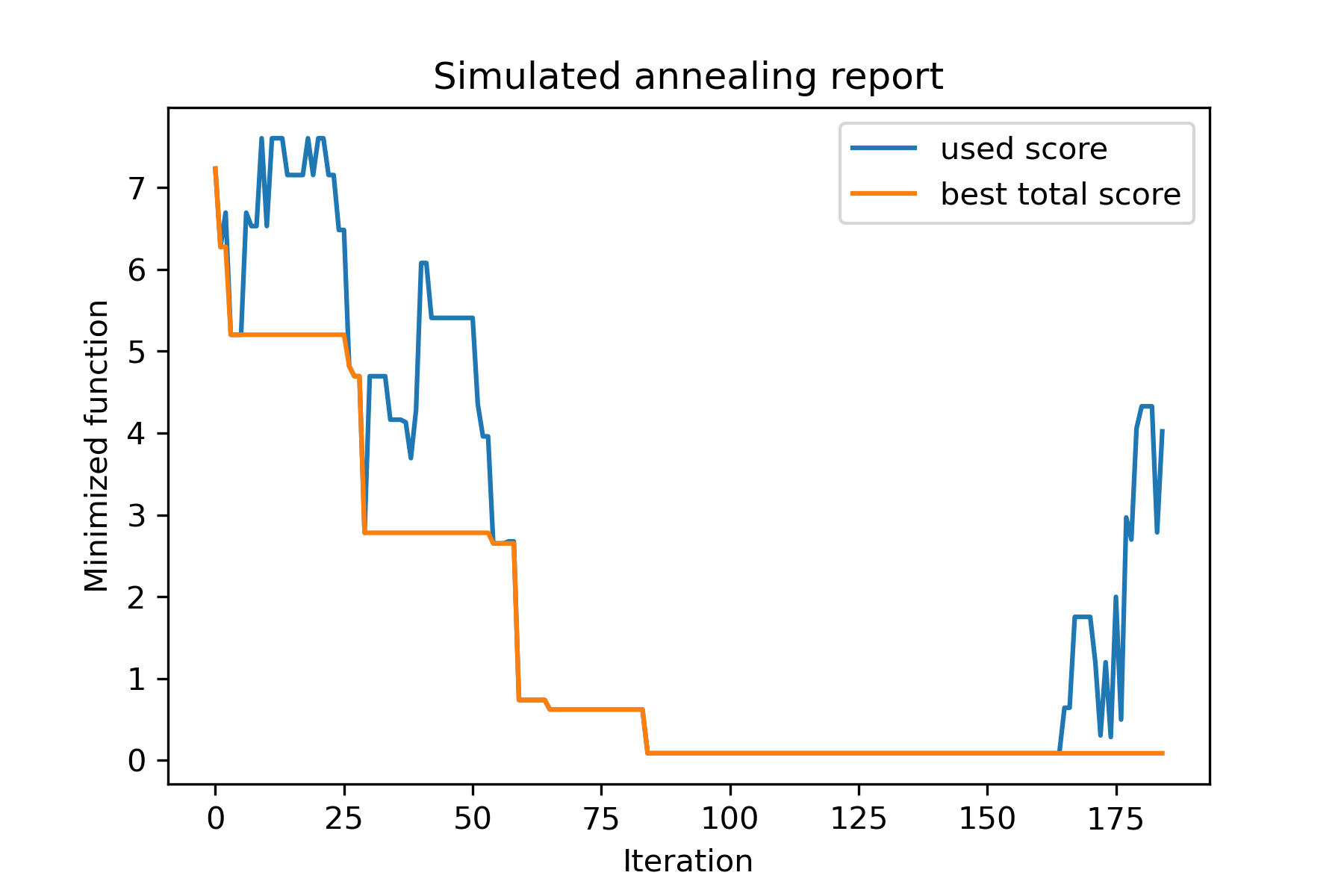
Schauen wir uns diese Aufgabe an:
 split set of values {v1, v2, v3, ..., vn} to sets 0, 1, 2, 3
with their sizes (volumes determined by user) to complete best sets metric
Eine Möglichkeit, es zu lösen:
 from collections import defaultdict
import numpy as np

from SimplestSimulatedAnnleaning import SimulatedAnnealing , Cooling

################### useful methods

def counts_to_vec ( dic_count ):
    """
    converts dictionary like {1: 3, 2: 4}
    to array [1, 1, 1, 2, 2, 2, 2]
    """
    arrs = [ np . full ( val , fill_value = key ) for key , val in dic_count . items ()]

    return np . concatenate ( tuple ( arrs ))

def vec_to_indexes_dict ( vector ):
    """
    converts vector like [1, 0, 1, 2, 2]
    to dictionary with indexes {1: [0, 2], 2: [3, 4]}
    """

    res = defaultdict ( list )

    for i , v in enumerate ( vector ):
        res [ v ]. append ( i )

    return { int ( key ): np . array ( val ) for key , val in res . items () if key != 0 }


#################### START PARAMS

SEED = 3

np . random . seed ( SEED )

Set = np . random . uniform ( low = - 15 , high = 5 , size = 100 ) # all set
Set_indexes = np . arange ( Set . size )

# how many objects should be in each set
dim_dict = {
    1 : 10 ,
    2 : 10 ,
    3 : 7 ,
    4 : 14
}


# minimized function: sum of means vy each split set
def min_func ( arr ):

    indexes_dict = vec_to_indexes_dict ( arr )

    means = [ np . mean ( Set [ val ]) for val in indexes_dict . values ()]

    return sum ( means )

# zero vector with available set labels at random positions
start_solution = np . zeros ( Set . size , dtype = np . int8 )
labels_vec = counts_to_vec ( dim_dict )
start_solution [ np . random . choice ( Set_indexes , labels_vec . size , replace = False )] = labels_vec


def choice ( count = 3 ):
    return np . random . choice ( Set_indexes , count , replace = False )

# mutation function
# temperature is the number cuz we will use only 1 cooling, but it's not necessary to use it)
def mut ( x_as_array , temperature_as_array_or_one_number ):

    new_x_as_array = x_as_array . copy ()
    # replace some values

    while True :
        inds = choice ()

        if np . unique ( new_x_as_array [ inds ]). size == 1 : # there is no sense to replace same values
            continue
        new_x_as_array [ inds ] = new_x_as_array [ np . random . permutation ( inds )]

        return new_x_as_array

# creating a model
model = SimulatedAnnealing ( min_func , Set_indexes . size )

# run search
best_solution , best_val = model . run (
    start_solution = start_solution ,
    mutation = mut ,
    cooling = Cooling . exponential ( 0.9 ),
    start_temperature = 100 ,
    max_function_evals = 1000 ,
    max_iterations_without_progress = 100 ,
    step_for_reinit_temperature = 80 ,
    seed = SEED ,
    reinit_from_best = True
    )

model . plot_report ( save_as = 'best_split.png' )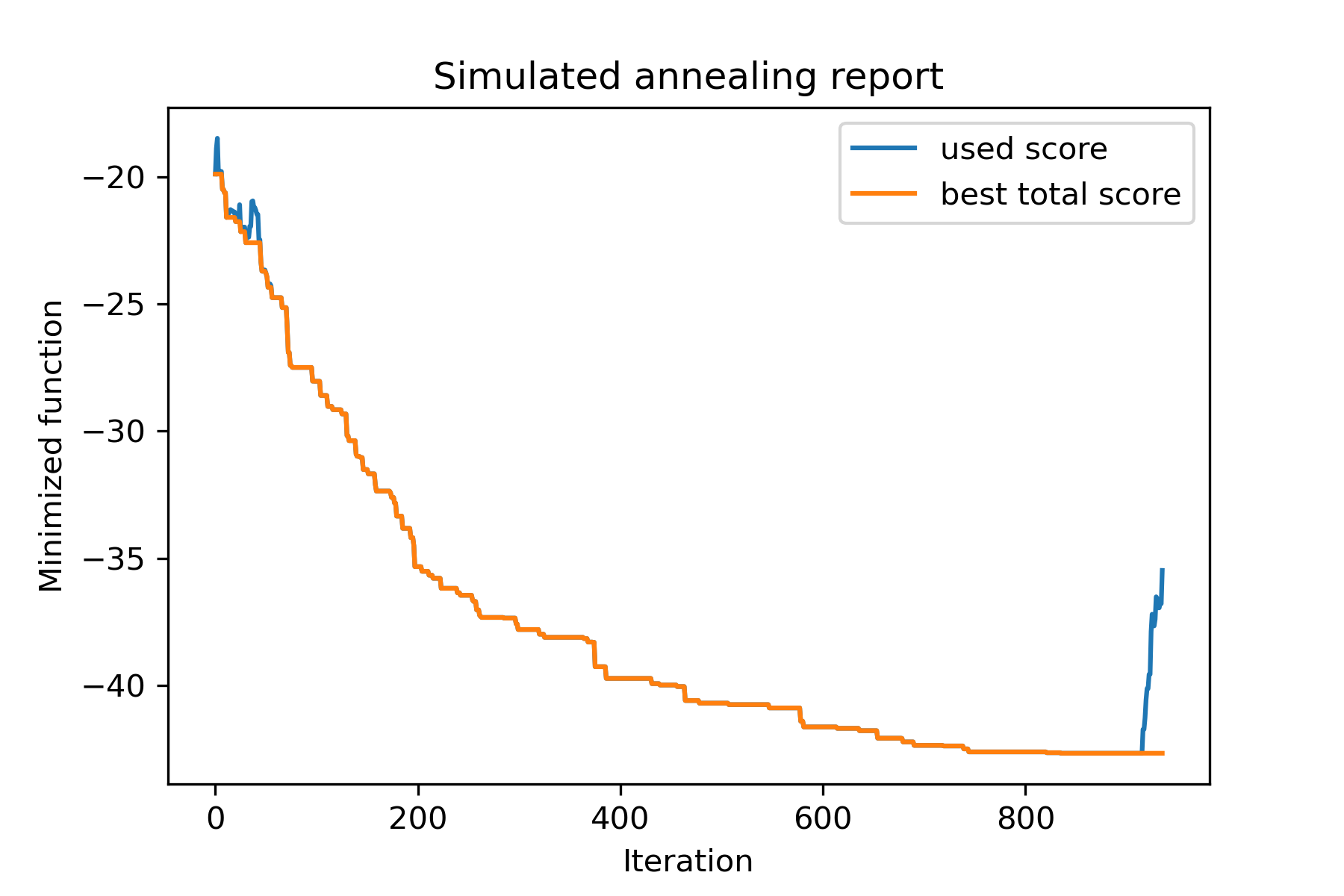
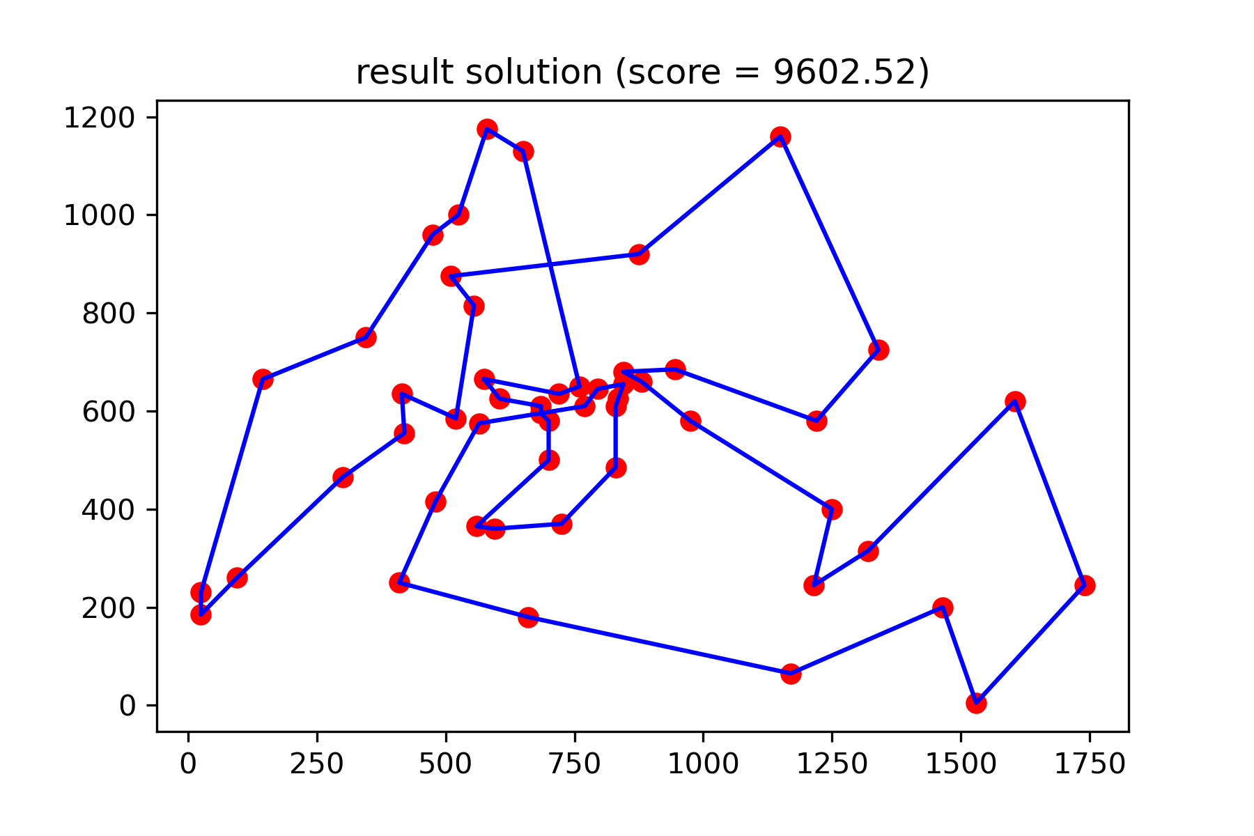
Versuchen wir, das Problem des reisenden Verkäufers für die Berlin52 -Aufgabe zu lösen. In dieser Aufgabe gibt es 52 Städte mit Koordinaten aus der Datei.
Lassen Sie uns zunächst Pakete importieren:
 import math
import numpy as np
import pandas as pd
import matplotlib . pyplot as plt

from SimplestSimulatedAnnleaning import SimulatedAnnealing , Cooling
Saatgut für die Reproduktion einstellen:
 SEED = 1
np . random . seed ( SEED )
Koordinaten lesen und Distanzmatrix erstellen:
 # read coordinates
coords = pd . read_csv ( 'berlin52_coords.txt' , sep = ' ' , header = None , names = [ 'index' , 'x' , 'y' ])

# dim is equal to count of cities
dim = coords . shape [ 0 ]

# distance matrix
distances = np . empty (( dim , dim ))

for i in range ( dim ):
    distances [ i , i ] = 0
    for j in range ( i + 1 , dim ):
        d = math . sqrt ( np . sum (( coords . iloc [ i , 1 :] - coords . iloc [ j , 1 :]) ** 2 ))
        distances [ i , j ] = d
        distances [ j , i ] = d
Erstellen Sie zufällige Startlösung:
 indexes = np . arange ( dim )
# some start solution (indexes shuffle)
start_solution = np . random . choice ( indexes , dim , replace = False )
Definieren Sie eine Funktion, die die Länge des Weges berechnet:
 # minized function
def way_length ( arr ):
    s = 0
    for i in range ( 1 , dim ):
        s += distances [ arr [ i - 1 ], arr [ i ]]
    # also we should end the way in the beggining
    s += distances [ arr [ - 1 ], arr [ 1 ]]

    return s
Lassen Sie uns die Startlösung visualisieren:
 def plotData ( indices , title , save_as = None ):

    # create a list of the corresponding city locations:
    locs = [ coords . iloc [ i , 1 :] for i in indices ]
    locs . append ( coords . iloc [ indices [ 0 ], 1 :])

    # plot a line between each pair of consequtive cities:
    plt . plot ( * zip ( * locs ), linestyle = '-' , color = 'blue' )

    # plot the dots representing the cities:
    plt . scatter ( coords . iloc [:, 1 ], coords . iloc [:, 2 ], marker = 'o' , s = 40 , color = 'red' )
    plt . title ( title )

    if not ( save_as is None ):  plt . savefig ( save_as , dpi = 300 )

    plt . show ()


# let's plot start solution
plotData ( start_solution , f'start random solution (score = { round ( way_length ( start_solution ), 2 ) } )' , 'salesman_start.png' )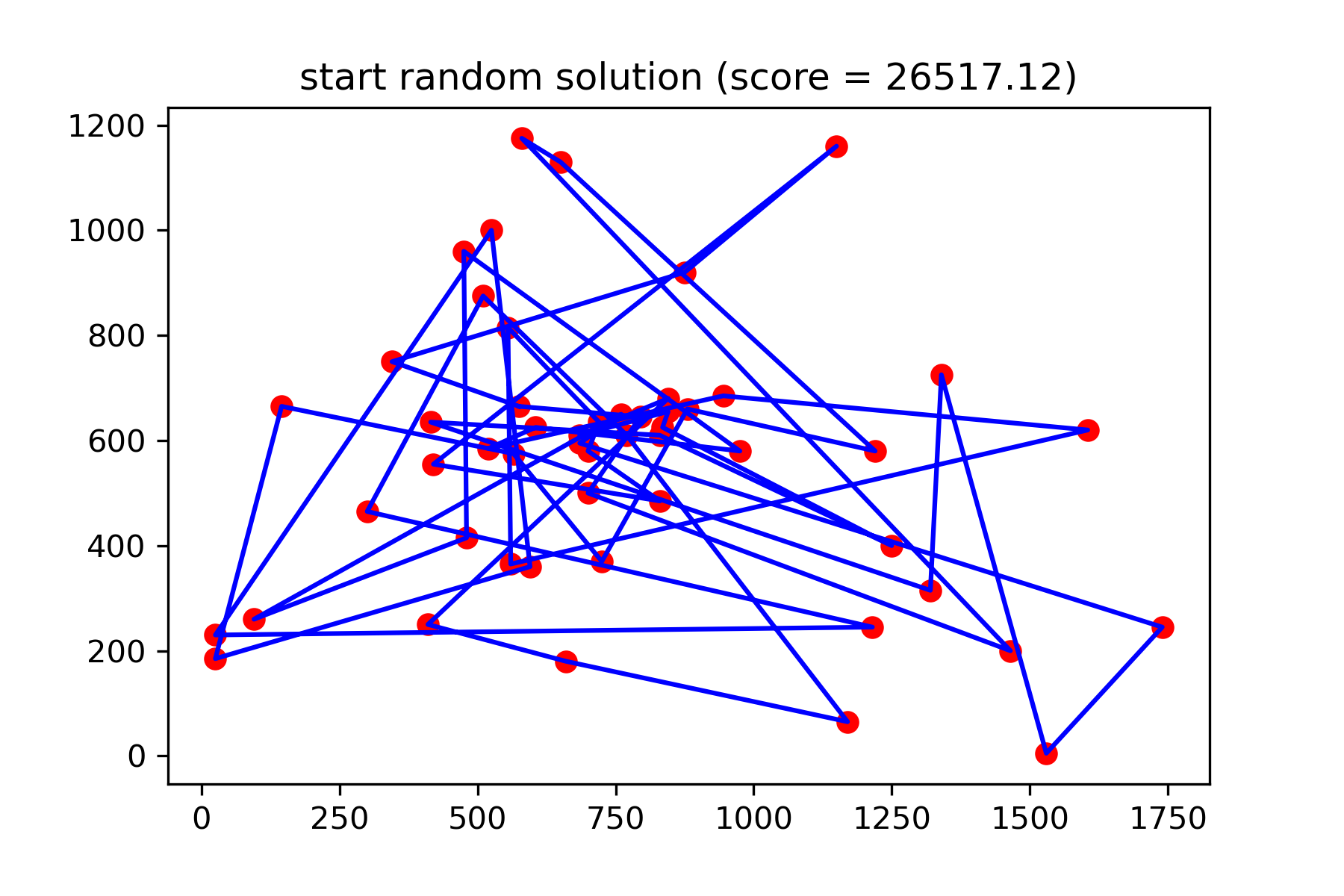
Es ist wirklich keine gute Lösung. Ich möchte diese Mutationsfunktion für diese Aufgabe erstellen:
 def mut ( x_as_array , temperature_as_array_or_one_number ):
    # random indexes
    rand_inds = np . random . choice ( indexes , 3 , replace = False )
    # shuffled indexes
    goes_to = np . random . permutation ( rand_inds )

    # just replace some positions in the array
    new_x_as_array = x_as_array . copy ()
    new_x_as_array [ rand_inds ] = new_x_as_array [ goes_to ]

    return new_x_as_array
Beginnen Sie mit der Suche:
 # creating a model
model = SimulatedAnnealing ( way_length , dim )

# run search
best_solution , best_val = model . run (
    start_solution = start_solution ,
    mutation = mut ,
    cooling = Cooling . exponential ( 0.9 ),
    start_temperature = 100 ,
    max_function_evals = 15000 ,
    max_iterations_without_progress = 2000 ,
    step_for_reinit_temperature = 80 ,
    reinit_from_best = True ,
    seed = SEED
    )

model . plot_report ( save_as = 'best_salesman.png' )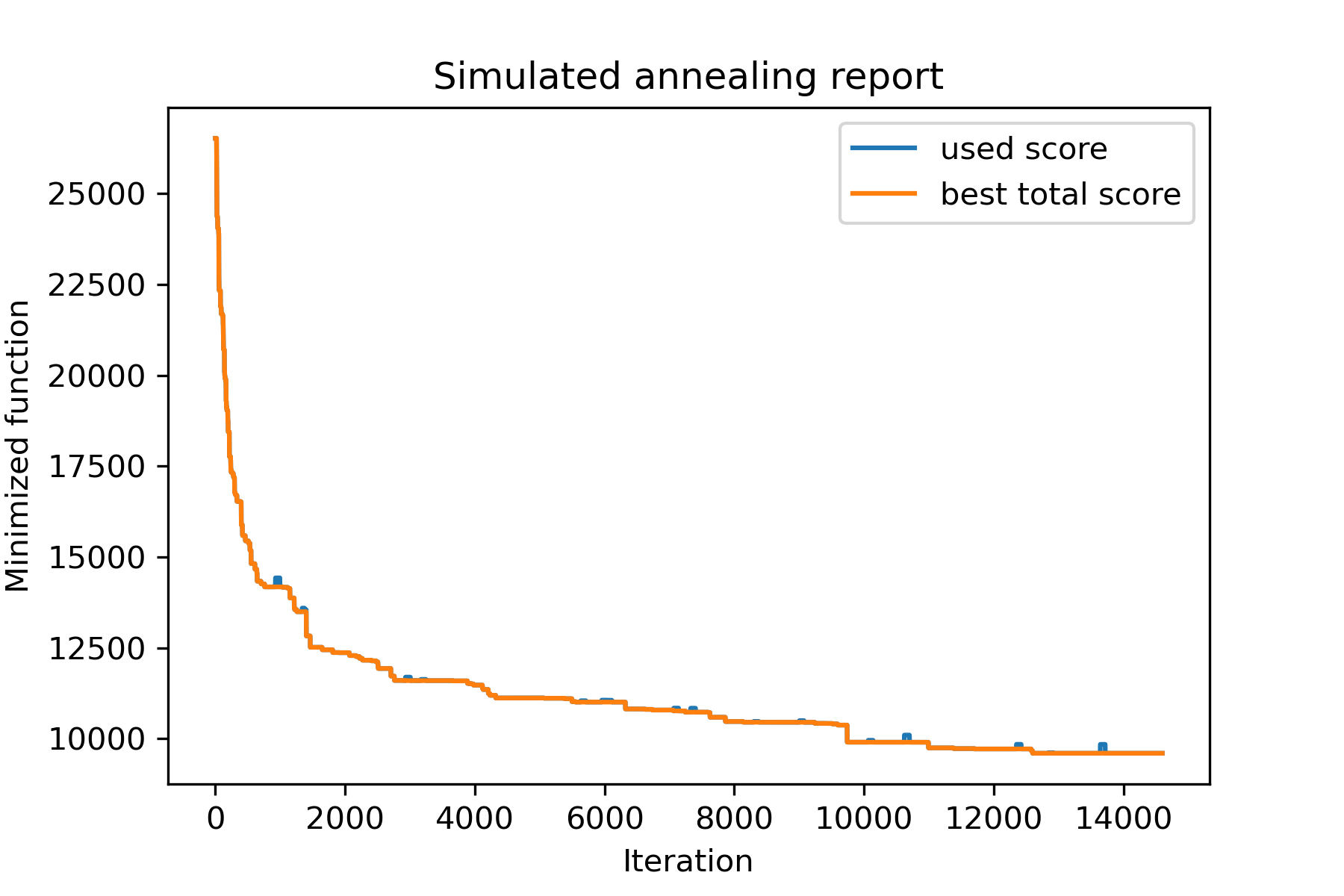
Und sehen Sie unsere viel bessere Lösung:
plotData ( best_solution , f'result solution (score = { round ( best_val , 2 ) } )' , 'salesman_result.png' )