SimplestSimulatedAnnealing
1.0.0
Implementación más simple (de DPEA) del método de recocido simulado
pip install SimplestSimulatedAnnealing
Este es el algoritmo evolutivo para la minimización de la función .
Pasos:
f debe minimizarsex0 (puede ser aleatorio)mut . Esta función debe dar una solución x1 nueva (puede ser aleatoria) utilizando información sobre x0 y temperatura T .cooling (comportamiento de temperatura)Tx0 y f(x0) mejor puntajex1 = mut(x0) y calculemos f(x1)f(x1) < f(x0) , encontramos una mejor solución x0 = x1 . De lo contrario, podemos reemplazar x1 con x0 con probabilidad igualizada exp((f(x0) - f(x1)) / T)T usando la función cooling : T = cooling(T)Paquetes de importación:
 import math
import numpy as np

from SimplestSimulatedAnnleaning import SimulatedAnnealing , Cooling , simple_continual_mutation
Determinar la función minimizada (rastrigin):
 def Rastrigin ( arr ):
    return 10 * arr . size + np . sum ( arr ** 2 ) - 10 * np . sum ( np . cos ( 2 * math . pi * arr ))

dim = 5
Usaremos la mutación Gauss más simple:
mut = simple_continual_mutation ( std = 0.5 )Crear objeto modelo (establecer función y dimensión):
model = SimulatedAnnealing ( Rastrigin , dim )Comience a buscar y vea el informe:
 best_solution , best_val = model . run (
    start_solution = np . random . uniform ( - 5 , 5 , dim ),
    mutation = mut ,
    cooling = Cooling . exponential ( 0.9 ),
    start_temperature = 100 ,
    max_function_evals = 1000 ,
    max_iterations_without_progress = 100 ,
    step_for_reinit_temperature = 80
    )

model . plot_report ( save_as = 'simple_example.png' )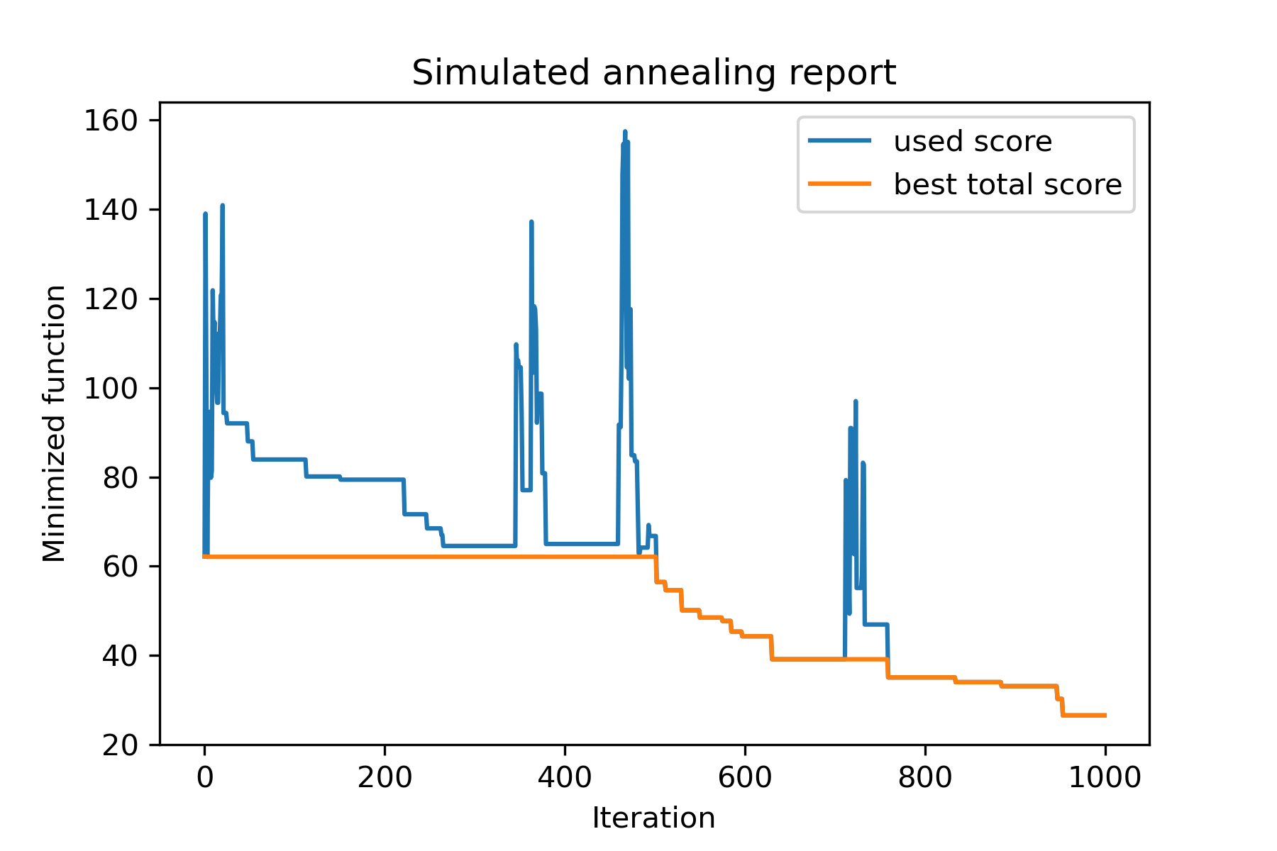
El método principal del paquete se run() . Vamos a ver sus argumentos:
 model . run ( start_solution ,
          mutation ,
          cooling ,
          start_temperature ,
          max_function_evals = 1000 ,
          max_iterations_without_progress = 250 ,
          step_for_reinit_temperature = 90 ,
          reinit_from_best = False ,
          seed = None )
Dónde:
start_solution : numpy array; solución de la que debe comenzar.
mutation : función (matriz, matriz/número). Funcionar como
 def mut ( x_as_array , temperature_as_array_or_one_number ):
    # some code
    return new_x_as_array
Esta función creará nuevas soluciones de existentes. Ver también
cooling : Función de enfriamiento / lista de funciones. Función de enfriamiento o una lista de otros. Ver
start_temperature : matriz de números o números (lista/tupla). Iniciar temperaturas. Puede ser un número o una variedad de números.
max_function_evals : int, opcional. Número máximo de evaluaciones de funciones. El valor predeterminado es 1000.
max_iterations_without_progress : int, opcional. Número máximo de iteraciones sin progreso global. El valor predeterminado es 250.
step_for_reinit_temperature : int, opcional. Después de este número de iteraciones sin progreso, las temperaturas se inicializarán como el inicio como el comienzo. El valor predeterminado es 90.
reinit_from_best : boolean, opcional. Inicie el algoritmo de la mejor solución después de las temperaturas de reinitamiento (o de la última solución de corriente). El valor predeterminado es falso.
seed : int/ninguno, opcional. Semilla aleatoria (si es necesario)
La parte importante del algoritmo es la función de enfriamiento . Esta función controla el valor de temperatura dependiendo del número de iteración actual, la temperatura de corriente y la temperatura de inicio. Puedes crear tu propia función de enfriamiento usando el patrón:
 def func ( T_last , T0 , k ):
    # some code
    return T_new
Aquí T_last (int/float) es el valor de temperatura de la iteración anterior, T0 (int/float) es la temperatura de inicio y k (int> 0) es el número de iteración. Debe usar parte de esta información para crear una nueva temperatura T_new .
Se recomienda construir su función para crear solo una temperatura positiva.
En la clase Cooling hay varias funciones de enfriamiento:
Cooling.linear(mu, Tmin = 0.01)Cooling.exponential(alpha = 0.9)Cooling.reverse(beta = 0.0005)Cooling.logarithmic(c, d = 1) - no recomendadoCooling.linear_reverse() Puede ver el comportamiento de la función de enfriamiento utilizando el método SimulatedAnnealing.plot_temperature . Veamos varios ejemplos:
 from SimplestSimulatedAnnleaning import SimulatedAnnealing , Cooling


# simplest way to set cooling regime
temperature = 100
cooling = Cooling . reverse ( beta = 0.001 )
# we can temperature behaviour using this code
SimulatedAnnealing . plot_temperature ( cooling , temperature , iterations = 100 , save_as = 'reverse.png' )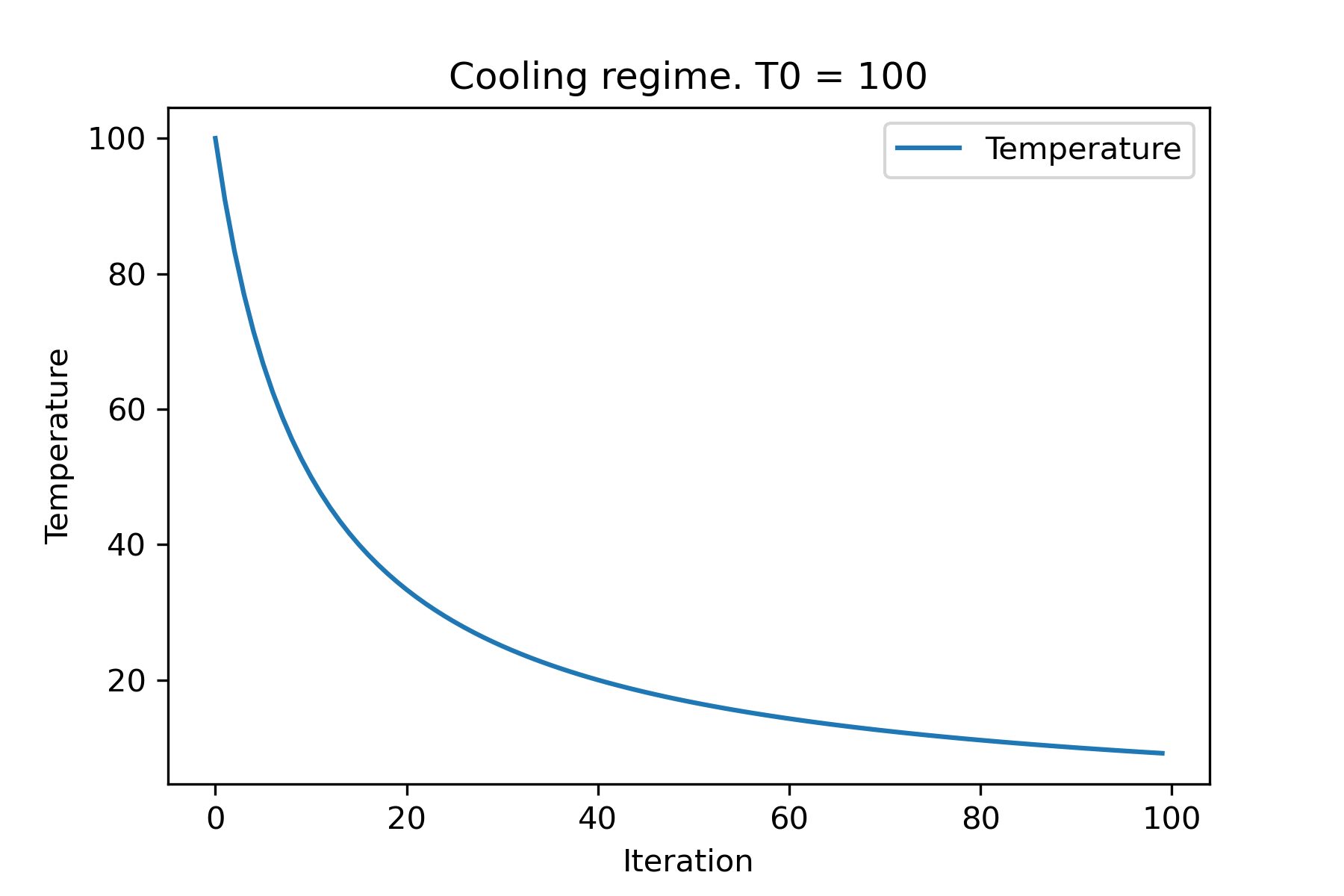
 # we can set several temparatures (for each dimention)
temperature = [ 150 , 100 , 50 ]
SimulatedAnnealing . plot_temperature ( cooling , temperature , iterations = 100 , save_as = 'reverse_diff_temp.png' )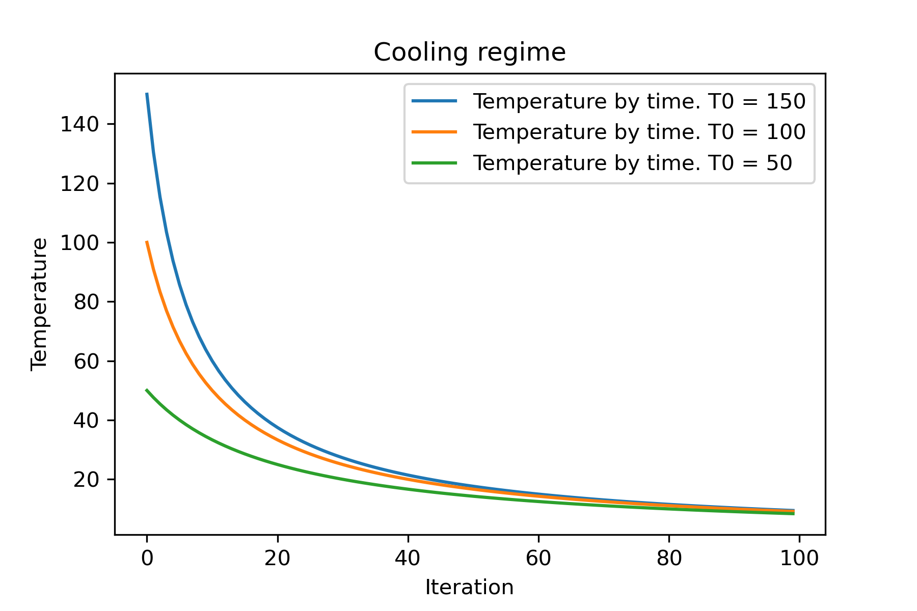
 # or several coolings (for each dimention)
temperature = 100
cooling = [
    Cooling . reverse ( beta = 0.0001 ),
    Cooling . reverse ( beta = 0.0005 ),
    Cooling . reverse ( beta = 0.001 )
    ]
SimulatedAnnealing . plot_temperature ( cooling , temperature , iterations = 100 , save_as = 'reverse_diff_beta.png' )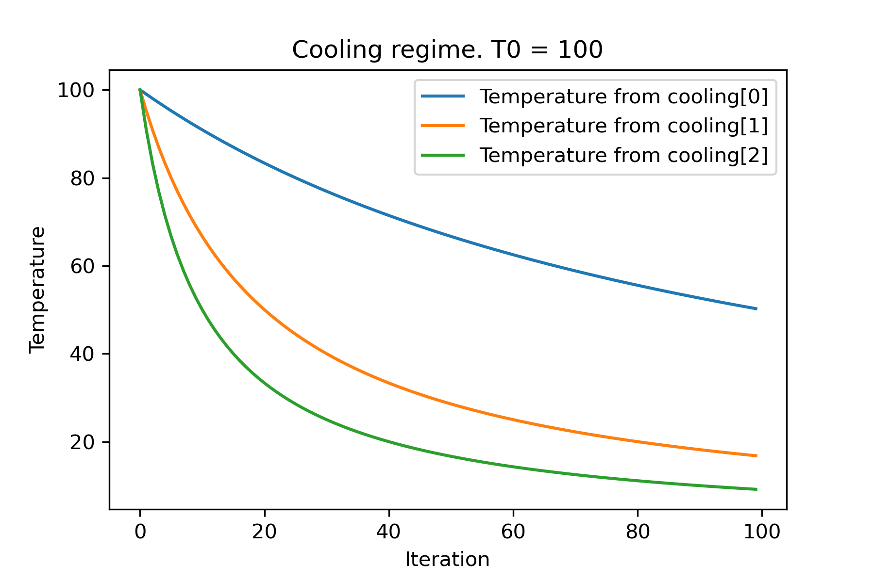
 # all supported coolling regimes

temperature = 100
cooling = [
    Cooling . linear ( mu = 1 ),
    Cooling . reverse ( beta = 0.0007 ),
    Cooling . exponential ( alpha = 0.85 ),
    Cooling . linear_reverse (),
    Cooling . logarithmic ( c = 100 , d = 1 )
    ]
SimulatedAnnealing . plot_temperature ( cooling , temperature , iterations = 100 , save_as = 'diff_temp.png' )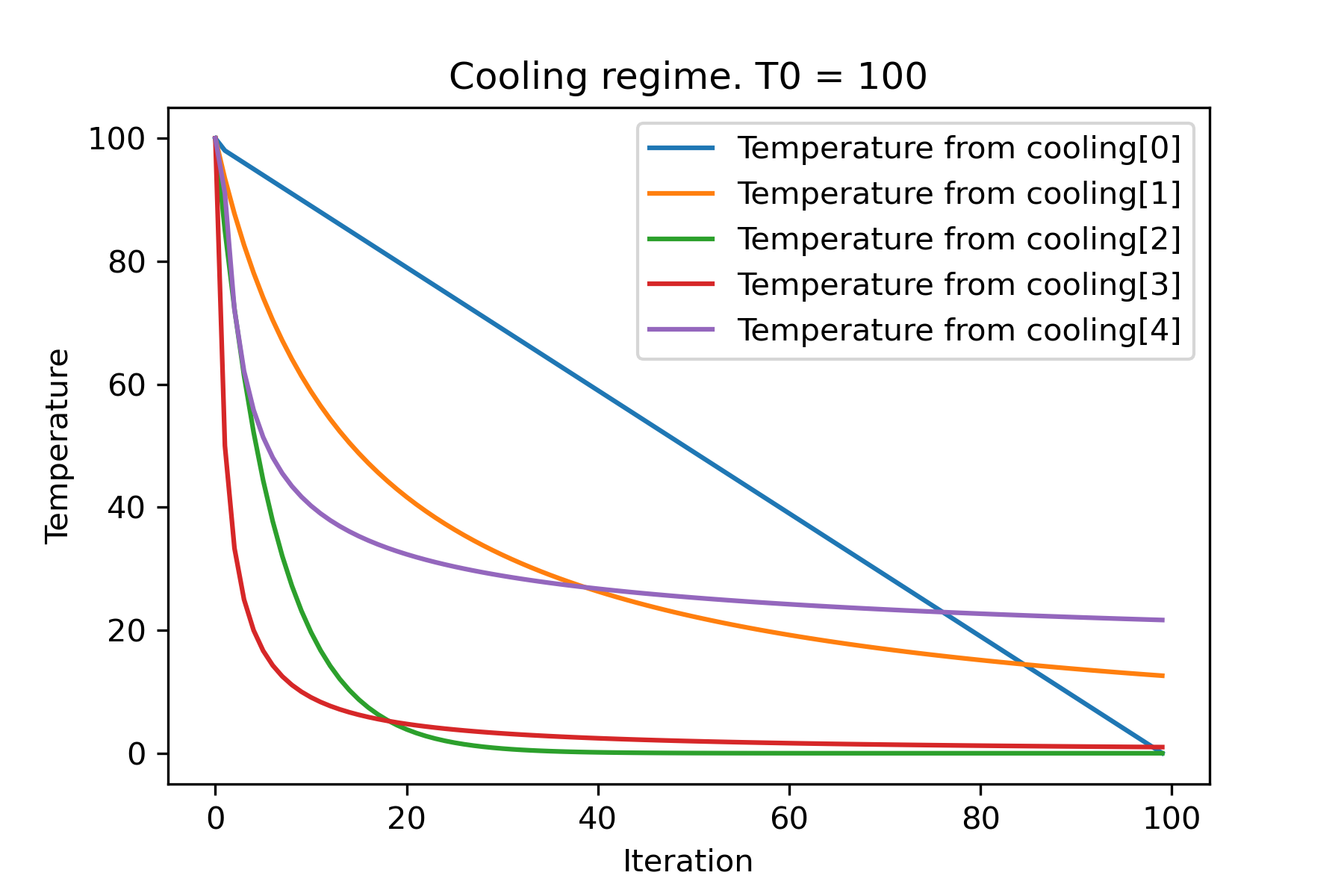
 # and we can set own temperature and cooling for each dimention!

temperature = [ 100 , 125 , 150 ]
cooling = [
    Cooling . exponential ( alpha = 0.85 ),
    Cooling . exponential ( alpha = 0.9 ),
    Cooling . exponential ( alpha = 0.95 ),
    ]
SimulatedAnnealing . plot_temperature ( cooling , temperature , iterations = 100 , save_as = 'diff_temp_and_cool.png' )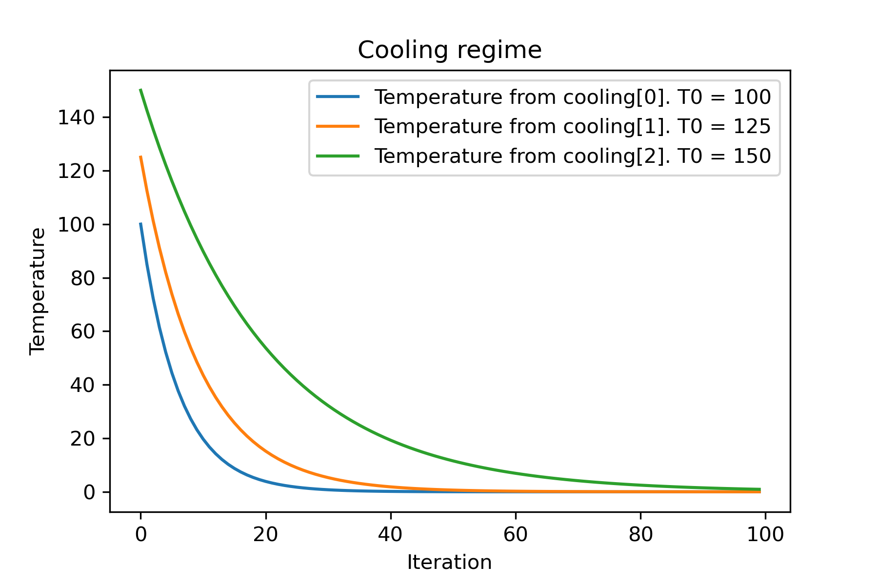
¿Por qué hay tantos regímenes de enfriamiento? ¡Para cierta tarea, uno de ellos puede ser tan mejor! En este script podemos probar diferentes enfriamientos para la función Rastring:
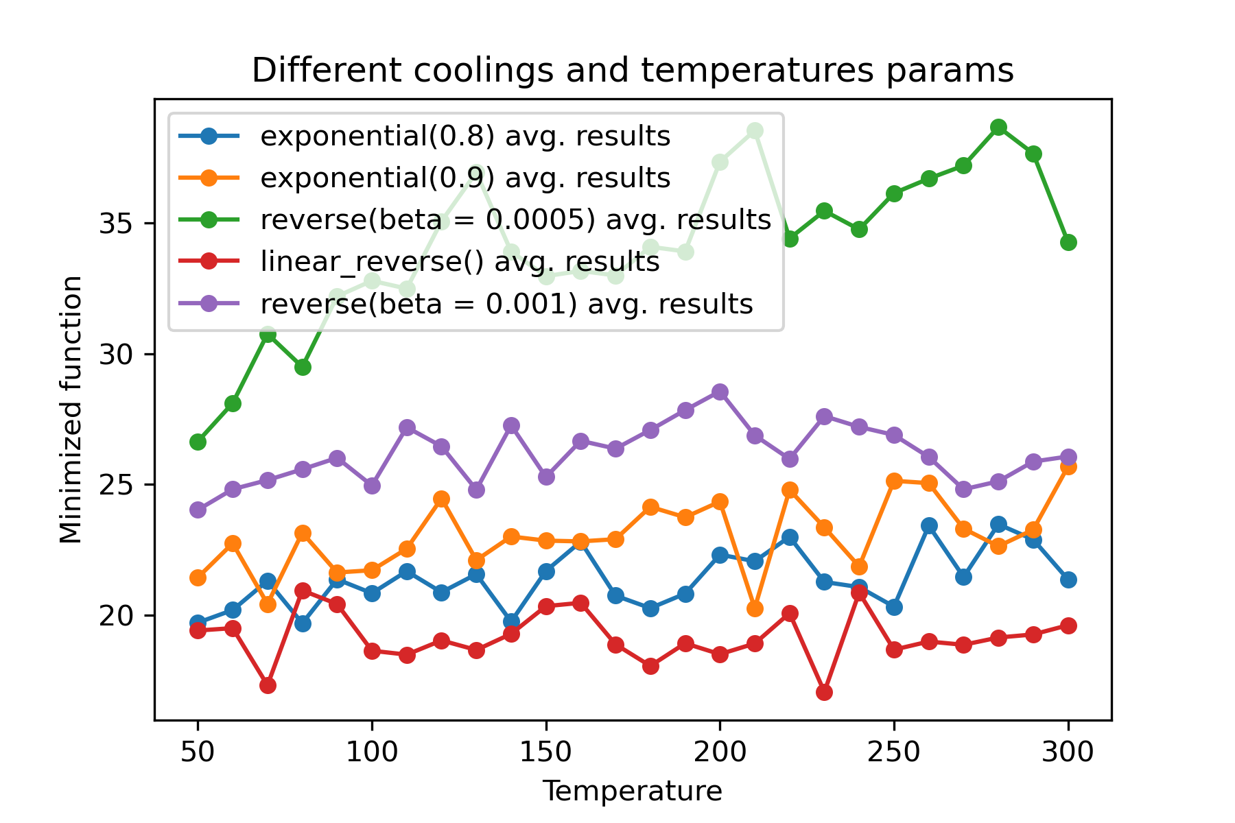
Es una característica sorprendente usar diferentes enfriamientos e inicio de temperaturas para cada dimensión :
 import math
import numpy as np

from SimplestSimulatedAnnleaning import SimulatedAnnealing , Cooling , simple_continual_mutation


def Rastrigin ( arr ):
    return 10 * arr . size + np . sum ( arr ** 2 ) - 10 * np . sum ( np . cos ( 2 * math . pi * arr ))

dim = 5


model = SimulatedAnnealing ( Rastrigin , dim )

best_solution , best_val = model . run (
    start_solution = np . random . uniform ( - 5 , 5 , dim ),
    mutation = simple_continual_mutation ( std = 1 ),
    cooling = [ # different cooling for each dimention
        Cooling . exponential ( 0.8 ),
        Cooling . exponential ( 0.9 ),
        Cooling . reverse ( beta = 0.0005 ),
        Cooling . linear_reverse (),
        Cooling . reverse ( beta = 0.001 )
        ],
    start_temperature = 100 ,
    max_function_evals = 1000 ,
    max_iterations_without_progress = 250 ,
    step_for_reinit_temperature = 90 ,
    reinit_from_best = False
    )

print ( best_val )

model . plot_report ( save_as = 'different_coolings.png' )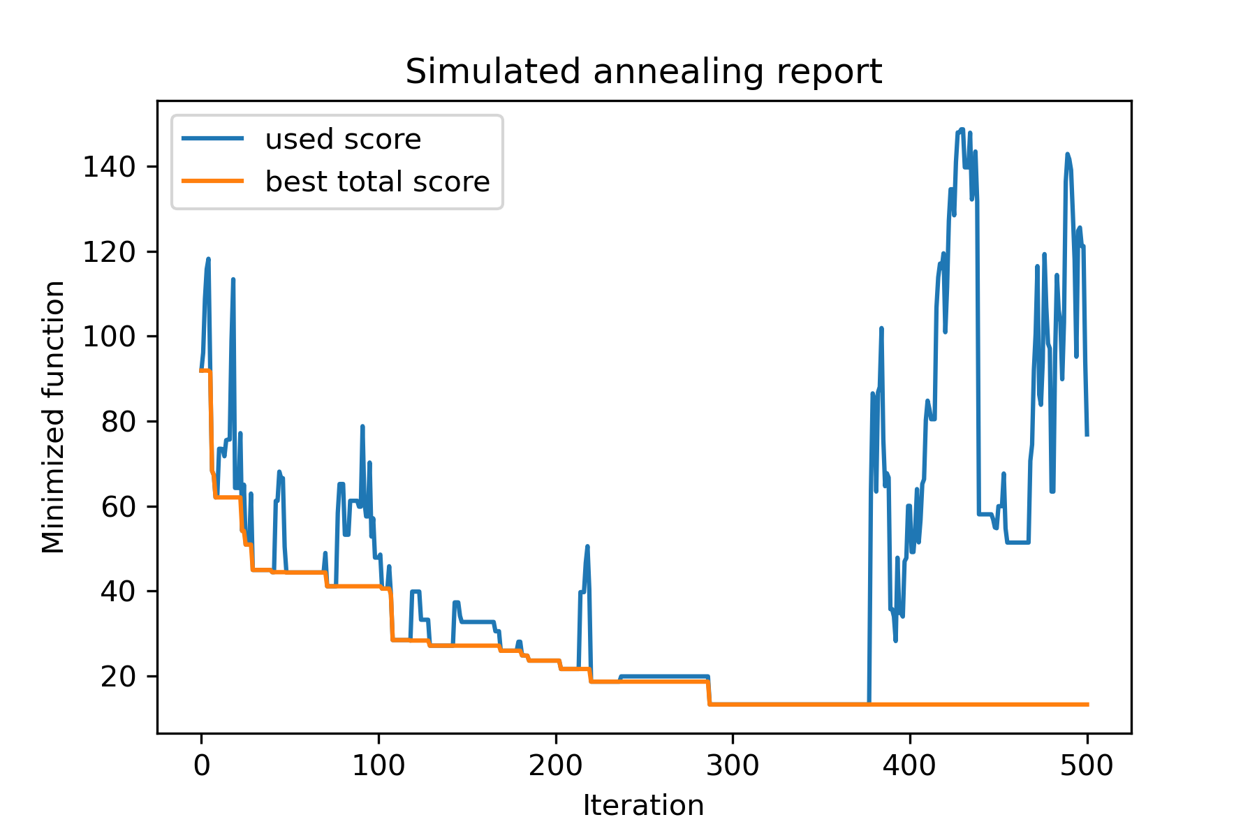
La razón principal para usar múltiples enfriamientos es el comportamiento de especificación de cada dimensión. Por ejemplo, la primera dimensión del espacio puede ser mucho más amplia que la segunda dimensión, por lo tanto, es mejor usar una búsqueda más amplia para la primera dimensión; Puede producirlo utilizando una función mut especial, utilizando diferentes start temperatures y usando diferentes coolings .
Otra razón para usar múltiples enfriamientos es la forma de selección: para la selección de múltiples enfriamientos entre soluciones buenas y malas aplicadas por cada dimensión . Entonces, aumenta las posibilidades de encontrar una mejor solución.
La función de mutación es el parámetro más importante. Determina el comportamiento de crear nuevos objetos utilizando información sobre el objeto actual y sobre la temperatura. Recomiendo contar estos principios al crear la función mut :
Recordemos la estructura de mut :
 def mut ( x_as_array , temperature_as_array_or_one_number ):
    # some code
    return new_x_as_array
Aquí x_as_array es la solución actual y new_x_as_array es la solución mutada (aleatoria y con el mismo tenue, como recuerdas). También debe recordar que temperature_as_array_or_one_number es el número solo para la solución de no maternidad. De lo contrario (cuando se usa varias temperaturas de inicio de varios enfriamientos o ambos) es una matriz numpy . Ver ejemplos
En este ejemplo, muestro cómo seleccionar los objetos k de SET con n objetos que minimizarán alguna función (en este ejemplo: Valor absoluto de la mediana):
 import numpy as np
from SimplestSimulatedAnnleaning import SimulatedAnnealing , Cooling

SEED = 3

np . random . seed ( SEED )

Set = np . random . uniform ( low = - 15 , high = 5 , size = 100 ) # all set

dim = 10 # how many objects should we choose

indexes = np . arange ( Set . size )
# minimized function -- subset with best |median|
def min_func ( arr ):
    return abs ( np . median ( Set [ indexes [ arr . astype ( bool )]]))

# zero vectors with 'dim' ones at random positions
start_solution = np . zeros ( Set . size )
start_solution [ np . random . choice ( indexes , dim , replace = False )] = 1

# mutation function
# temperature is the number cuz we will use only 1 cooling, but it's not necessary to use it)
def mut ( x_as_array , temperature_as_array_or_one_number ):
    mask_one = x_as_array == 1
    mask_zero = np . logical_not ( mask_one )

    new_x_as_array = x_as_array . copy ()
    # replace some zeros with ones
    new_x_as_array [ np . random . choice ( indexes [ mask_one ], 1 , replace = False )] = 0
    new_x_as_array [ np . random . choice ( indexes [ mask_zero ], 1 , replace = False )] = 1

    return new_x_as_array

# creating a model
model = SimulatedAnnealing ( min_func , dim )

# run search
best_solution , best_val = model . run (
    start_solution = start_solution ,
    mutation = mut ,
    cooling = Cooling . exponential ( 0.9 ),
    start_temperature = 100 ,
    max_function_evals = 1000 ,
    max_iterations_without_progress = 100 ,
    step_for_reinit_temperature = 80 ,
    seed = SEED
    )

model . plot_report ( save_as = 'best_subset.png' )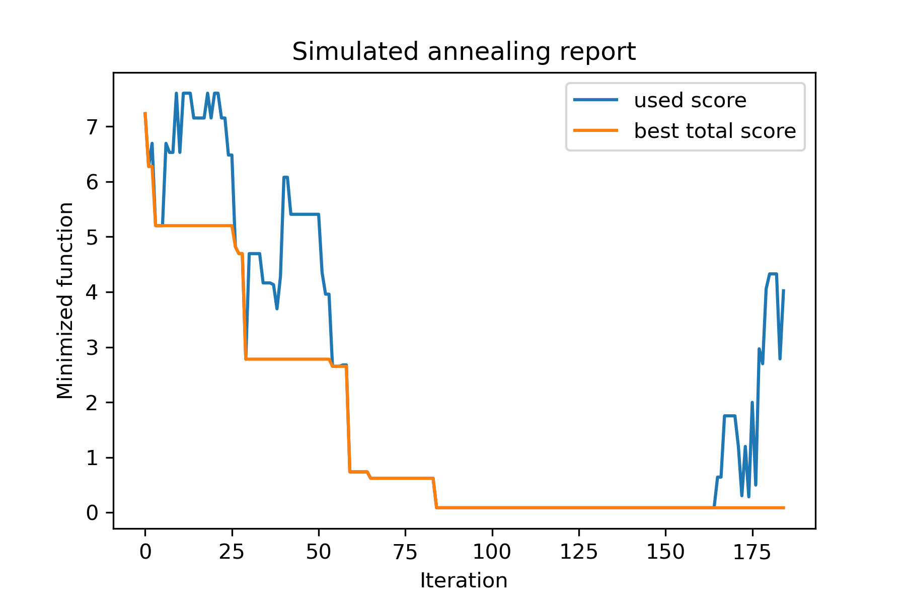
Echemos un vistazo a esta tarea:
 split set of values {v1, v2, v3, ..., vn} to sets 0, 1, 2, 3
with their sizes (volumes determined by user) to complete best sets metric
Una de las formas de resolverlo:
 from collections import defaultdict
import numpy as np

from SimplestSimulatedAnnleaning import SimulatedAnnealing , Cooling

################### useful methods

def counts_to_vec ( dic_count ):
    """
    converts dictionary like {1: 3, 2: 4}
    to array [1, 1, 1, 2, 2, 2, 2]
    """
    arrs = [ np . full ( val , fill_value = key ) for key , val in dic_count . items ()]

    return np . concatenate ( tuple ( arrs ))

def vec_to_indexes_dict ( vector ):
    """
    converts vector like [1, 0, 1, 2, 2]
    to dictionary with indexes {1: [0, 2], 2: [3, 4]}
    """

    res = defaultdict ( list )

    for i , v in enumerate ( vector ):
        res [ v ]. append ( i )

    return { int ( key ): np . array ( val ) for key , val in res . items () if key != 0 }


#################### START PARAMS

SEED = 3

np . random . seed ( SEED )

Set = np . random . uniform ( low = - 15 , high = 5 , size = 100 ) # all set
Set_indexes = np . arange ( Set . size )

# how many objects should be in each set
dim_dict = {
    1 : 10 ,
    2 : 10 ,
    3 : 7 ,
    4 : 14
}


# minimized function: sum of means vy each split set
def min_func ( arr ):

    indexes_dict = vec_to_indexes_dict ( arr )

    means = [ np . mean ( Set [ val ]) for val in indexes_dict . values ()]

    return sum ( means )

# zero vector with available set labels at random positions
start_solution = np . zeros ( Set . size , dtype = np . int8 )
labels_vec = counts_to_vec ( dim_dict )
start_solution [ np . random . choice ( Set_indexes , labels_vec . size , replace = False )] = labels_vec


def choice ( count = 3 ):
    return np . random . choice ( Set_indexes , count , replace = False )

# mutation function
# temperature is the number cuz we will use only 1 cooling, but it's not necessary to use it)
def mut ( x_as_array , temperature_as_array_or_one_number ):

    new_x_as_array = x_as_array . copy ()
    # replace some values

    while True :
        inds = choice ()

        if np . unique ( new_x_as_array [ inds ]). size == 1 : # there is no sense to replace same values
            continue
        new_x_as_array [ inds ] = new_x_as_array [ np . random . permutation ( inds )]

        return new_x_as_array

# creating a model
model = SimulatedAnnealing ( min_func , Set_indexes . size )

# run search
best_solution , best_val = model . run (
    start_solution = start_solution ,
    mutation = mut ,
    cooling = Cooling . exponential ( 0.9 ),
    start_temperature = 100 ,
    max_function_evals = 1000 ,
    max_iterations_without_progress = 100 ,
    step_for_reinit_temperature = 80 ,
    seed = SEED ,
    reinit_from_best = True
    )

model . plot_report ( save_as = 'best_split.png' )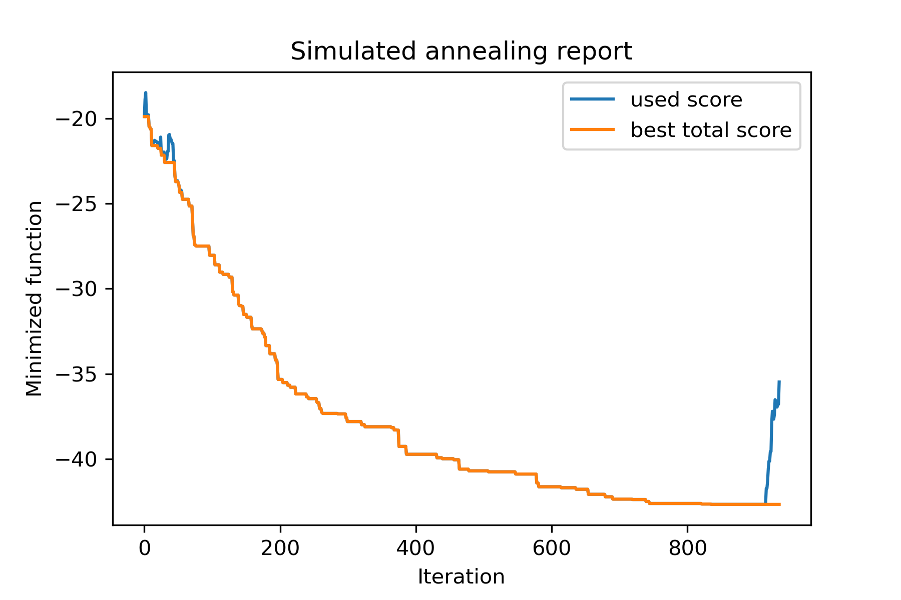
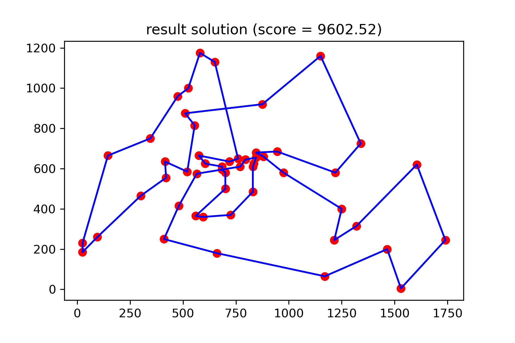
Intentemos resolver el problema de los vendedores viajeros para la tarea Berlin52. En esta tarea hay 52 ciudades con coordenadas del archivo.
En primer lugar, importemos paquetes:
 import math
import numpy as np
import pandas as pd
import matplotlib . pyplot as plt

from SimplestSimulatedAnnleaning import SimulatedAnnealing , Cooling
Establecer semilla para reproducir:
 SEED = 1
np . random . seed ( SEED )
Leer coordenadas y crear matriz de distancia:
 # read coordinates
coords = pd . read_csv ( 'berlin52_coords.txt' , sep = ' ' , header = None , names = [ 'index' , 'x' , 'y' ])

# dim is equal to count of cities
dim = coords . shape [ 0 ]

# distance matrix
distances = np . empty (( dim , dim ))

for i in range ( dim ):
    distances [ i , i ] = 0
    for j in range ( i + 1 , dim ):
        d = math . sqrt ( np . sum (( coords . iloc [ i , 1 :] - coords . iloc [ j , 1 :]) ** 2 ))
        distances [ i , j ] = d
        distances [ j , i ] = d
Crear solución de inicio aleatorio:
 indexes = np . arange ( dim )
# some start solution (indexes shuffle)
start_solution = np . random . choice ( indexes , dim , replace = False )
Definir una función que calcula la longitud de camino:
 # minized function
def way_length ( arr ):
    s = 0
    for i in range ( 1 , dim ):
        s += distances [ arr [ i - 1 ], arr [ i ]]
    # also we should end the way in the beggining
    s += distances [ arr [ - 1 ], arr [ 1 ]]

    return s
Visualizemos la solución de inicio:
 def plotData ( indices , title , save_as = None ):

    # create a list of the corresponding city locations:
    locs = [ coords . iloc [ i , 1 :] for i in indices ]
    locs . append ( coords . iloc [ indices [ 0 ], 1 :])

    # plot a line between each pair of consequtive cities:
    plt . plot ( * zip ( * locs ), linestyle = '-' , color = 'blue' )

    # plot the dots representing the cities:
    plt . scatter ( coords . iloc [:, 1 ], coords . iloc [:, 2 ], marker = 'o' , s = 40 , color = 'red' )
    plt . title ( title )

    if not ( save_as is None ):  plt . savefig ( save_as , dpi = 300 )

    plt . show ()


# let's plot start solution
plotData ( start_solution , f'start random solution (score = { round ( way_length ( start_solution ), 2 ) } )' , 'salesman_start.png' )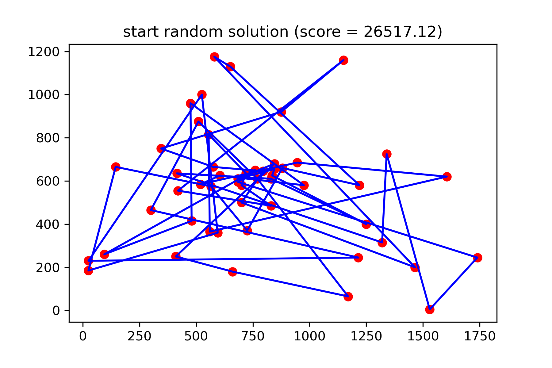
Realmente no es una buena solución. Quiero crear esta función de mutación para esta tarea:
 def mut ( x_as_array , temperature_as_array_or_one_number ):
    # random indexes
    rand_inds = np . random . choice ( indexes , 3 , replace = False )
    # shuffled indexes
    goes_to = np . random . permutation ( rand_inds )

    # just replace some positions in the array
    new_x_as_array = x_as_array . copy ()
    new_x_as_array [ rand_inds ] = new_x_as_array [ goes_to ]

    return new_x_as_array
Empiece a buscar:
 # creating a model
model = SimulatedAnnealing ( way_length , dim )

# run search
best_solution , best_val = model . run (
    start_solution = start_solution ,
    mutation = mut ,
    cooling = Cooling . exponential ( 0.9 ),
    start_temperature = 100 ,
    max_function_evals = 15000 ,
    max_iterations_without_progress = 2000 ,
    step_for_reinit_temperature = 80 ,
    reinit_from_best = True ,
    seed = SEED
    )

model . plot_report ( save_as = 'best_salesman.png' )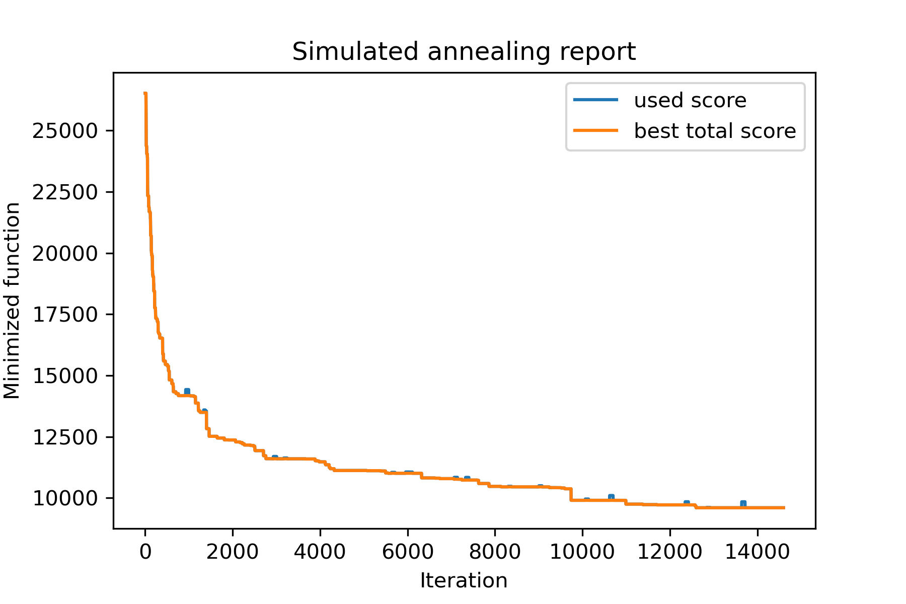
Y vea nuestra solución mucho mejor:
plotData ( best_solution , f'result solution (score = { round ( best_val , 2 ) } )' , 'salesman_result.png' )