SimplestSimulatedAnnealing
1.0.0
Implementação mais simples (do DPEA) do método de recozimento simulado
pip install SimplestSimulatedAnnealing
Este é o algoritmo evolutivo para a minimização da função .
Passos:
f deve ser minimizadax0 (pode ser aleatório)mut . Esta função deve fornecer uma solução x1 nova (pode ser aleatória) usando informações sobre x0 e temperatura T .cooling (comportamento da temperatura)Tx0 e a melhor pontuação f(x0)x1 = mut(x0) e calcular f(x1)f(x1) < f(x0) , encontramos melhor solução x0 = x1 . Caso contrário, podemos substituir x1 por x0 por probabilidade igual exp((f(x0) - f(x1)) / T)T usando a função cooling : T = cooling(T)Importar pacotes:
 import math
import numpy as np

from SimplestSimulatedAnnleaning import SimulatedAnnealing , Cooling , simple_continual_mutation
Determinar a função minimizada (rastrigin):
 def Rastrigin ( arr ):
    return 10 * arr . size + np . sum ( arr ** 2 ) - 10 * np . sum ( np . cos ( 2 * math . pi * arr ))

dim = 5
Usaremos a mutação Gauss mais simples:
mut = simple_continual_mutation ( std = 0.5 )Crie objeto de modelo (Definir função e dimensão):
model = SimulatedAnnealing ( Rastrigin , dim )Comece a pesquisar e consulte o relatório:
 best_solution , best_val = model . run (
    start_solution = np . random . uniform ( - 5 , 5 , dim ),
    mutation = mut ,
    cooling = Cooling . exponential ( 0.9 ),
    start_temperature = 100 ,
    max_function_evals = 1000 ,
    max_iterations_without_progress = 100 ,
    step_for_reinit_temperature = 80
    )

model . plot_report ( save_as = 'simple_example.png' )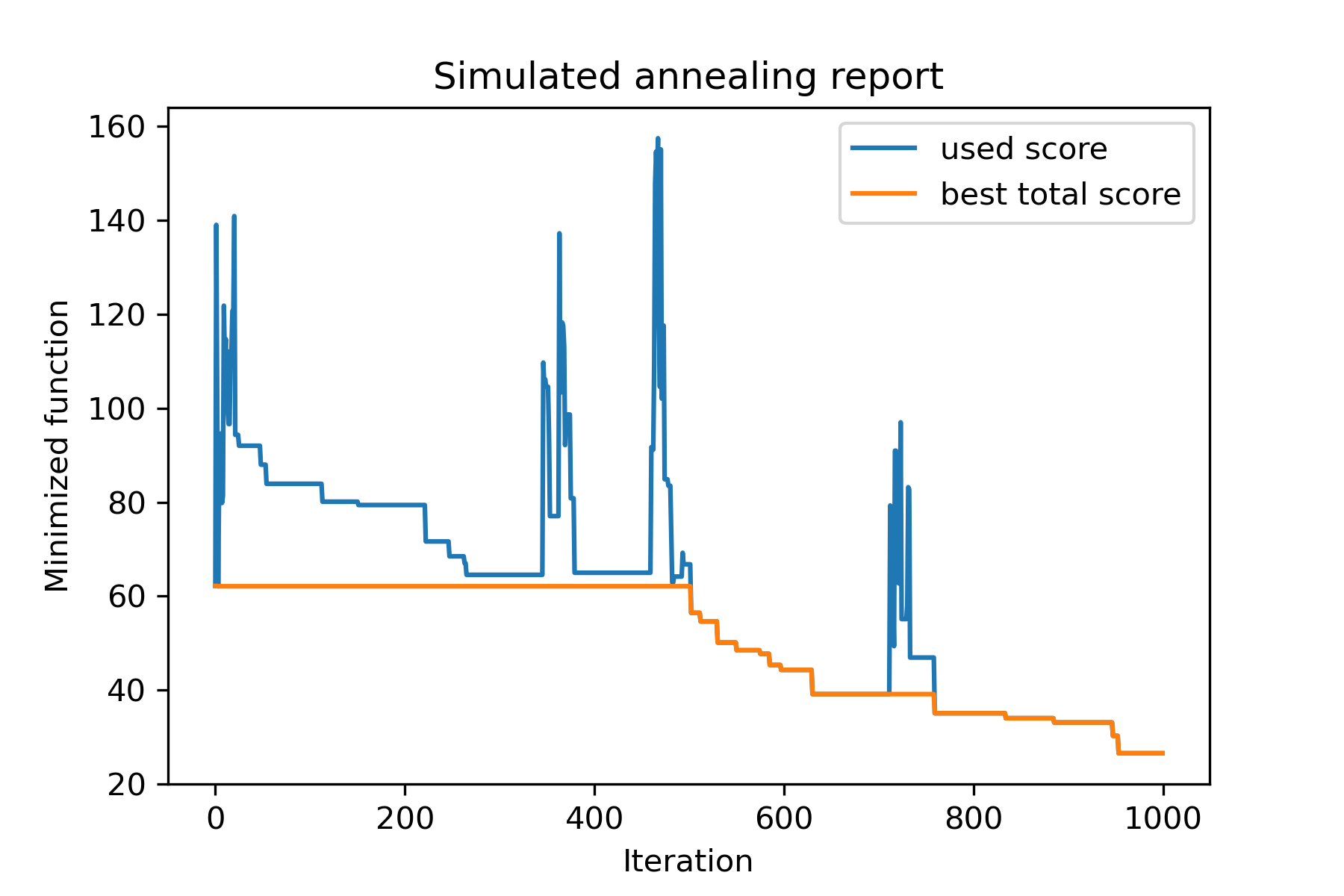
O método principal do pacote é run() . Vamos verificar seus argumentos:
 model . run ( start_solution ,
          mutation ,
          cooling ,
          start_temperature ,
          max_function_evals = 1000 ,
          max_iterations_without_progress = 250 ,
          step_for_reinit_temperature = 90 ,
          reinit_from_best = False ,
          seed = None )
Onde:
start_solution : Numpy Array; solução a partir da qual deve começar.
mutation : função (matriz, matriz/número). Função como
 def mut ( x_as_array , temperature_as_array_or_one_number ):
    # some code
    return new_x_as_array
Esta função criará novas soluções a partir de existentes. Veja também
cooling : Lista de funções / funções de resfriamento. Função de resfriamento ou uma lista de outras. Ver
start_temperature : matriz de número ou número (lista/tupla). Iniciar temperaturas. Pode ser um número ou uma variedade de números.
max_function_evals : int, opcional. Número máximo de avaliações de função. O padrão é 1000.
max_iterations_without_progress : int, opcional. Número máximo de iterações sem progresso global. O padrão é 250.
step_for_reinit_temperature : int, opcional. Após esse número de iterações sem o progresso, as temperaturas serão inicializadas como Start. O padrão é 90.
reinit_from_best : booleano, opcional. Inicie o algoritmo da melhor solução após reiniciar as temperaturas (ou da última solução atual). O padrão é falso.
seed : Int/Nenhum, opcional. Semente aleatória (se necessário)
A parte importante do algoritmo é a função de resfriamento . Esta função controla o valor da temperatura dependia do número da iteração da corrente, da temperatura da corrente e da temperatura inicial. Você pode criar sua própria função de refrigeração usando o padrão:
 def func ( T_last , T0 , k ):
    # some code
    return T_new
Aqui T_last (INT/FLOAT) é o valor da temperatura da iteração anterior, T0 (Int/Float) é a temperatura inicial e k (int> 0) é o número de iteração. Você deve usar algumas dessas informações para criar uma nova temperatura T_new .
É altamente recomendável construir sua função para criar apenas temperatura positiva.
Na aula Cooling , existem várias funções de resfriamento:
Cooling.linear(mu, Tmin = 0.01)Cooling.exponential(alpha = 0.9)Cooling.reverse(beta = 0.0005)Cooling.logarithmic(c, d = 1) - não recomendadoCooling.linear_reverse() U pode ver o comportamento da função de resfriamento usando o método SimulatedAnnealing.plot_temperature . Vamos ver vários exemplos:
 from SimplestSimulatedAnnleaning import SimulatedAnnealing , Cooling


# simplest way to set cooling regime
temperature = 100
cooling = Cooling . reverse ( beta = 0.001 )
# we can temperature behaviour using this code
SimulatedAnnealing . plot_temperature ( cooling , temperature , iterations = 100 , save_as = 'reverse.png' )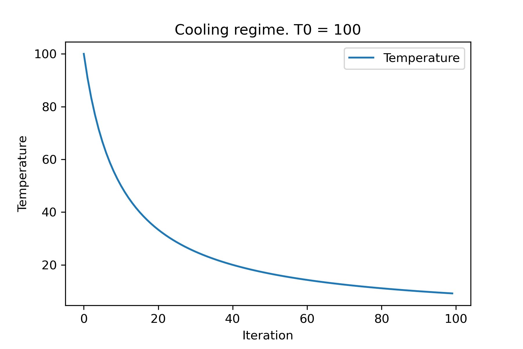
 # we can set several temparatures (for each dimention)
temperature = [ 150 , 100 , 50 ]
SimulatedAnnealing . plot_temperature ( cooling , temperature , iterations = 100 , save_as = 'reverse_diff_temp.png' )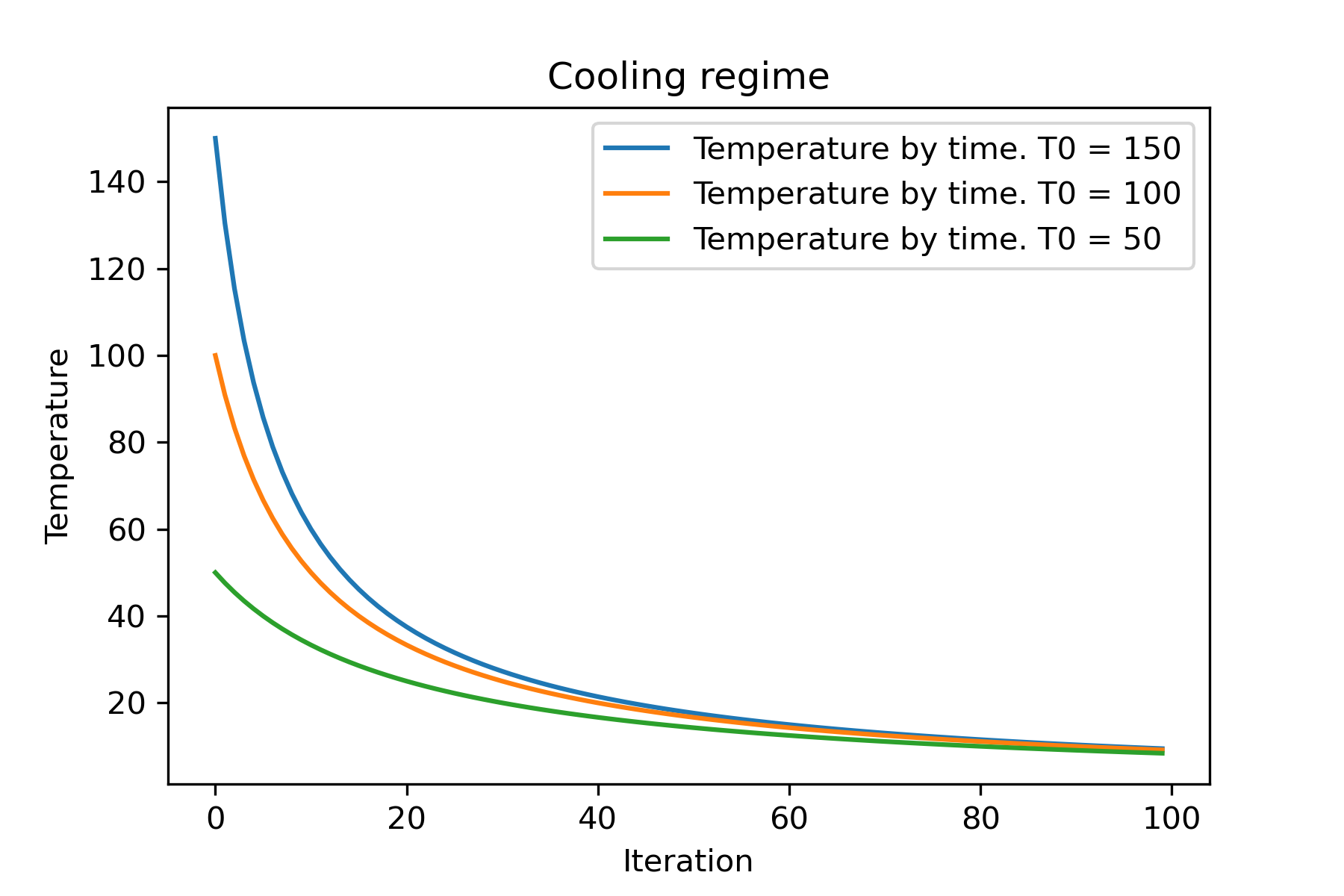
 # or several coolings (for each dimention)
temperature = 100
cooling = [
    Cooling . reverse ( beta = 0.0001 ),
    Cooling . reverse ( beta = 0.0005 ),
    Cooling . reverse ( beta = 0.001 )
    ]
SimulatedAnnealing . plot_temperature ( cooling , temperature , iterations = 100 , save_as = 'reverse_diff_beta.png' )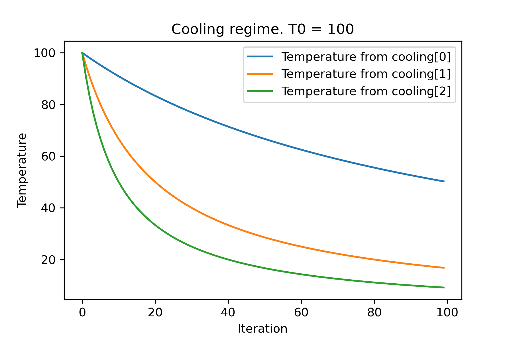
 # all supported coolling regimes

temperature = 100
cooling = [
    Cooling . linear ( mu = 1 ),
    Cooling . reverse ( beta = 0.0007 ),
    Cooling . exponential ( alpha = 0.85 ),
    Cooling . linear_reverse (),
    Cooling . logarithmic ( c = 100 , d = 1 )
    ]
SimulatedAnnealing . plot_temperature ( cooling , temperature , iterations = 100 , save_as = 'diff_temp.png' )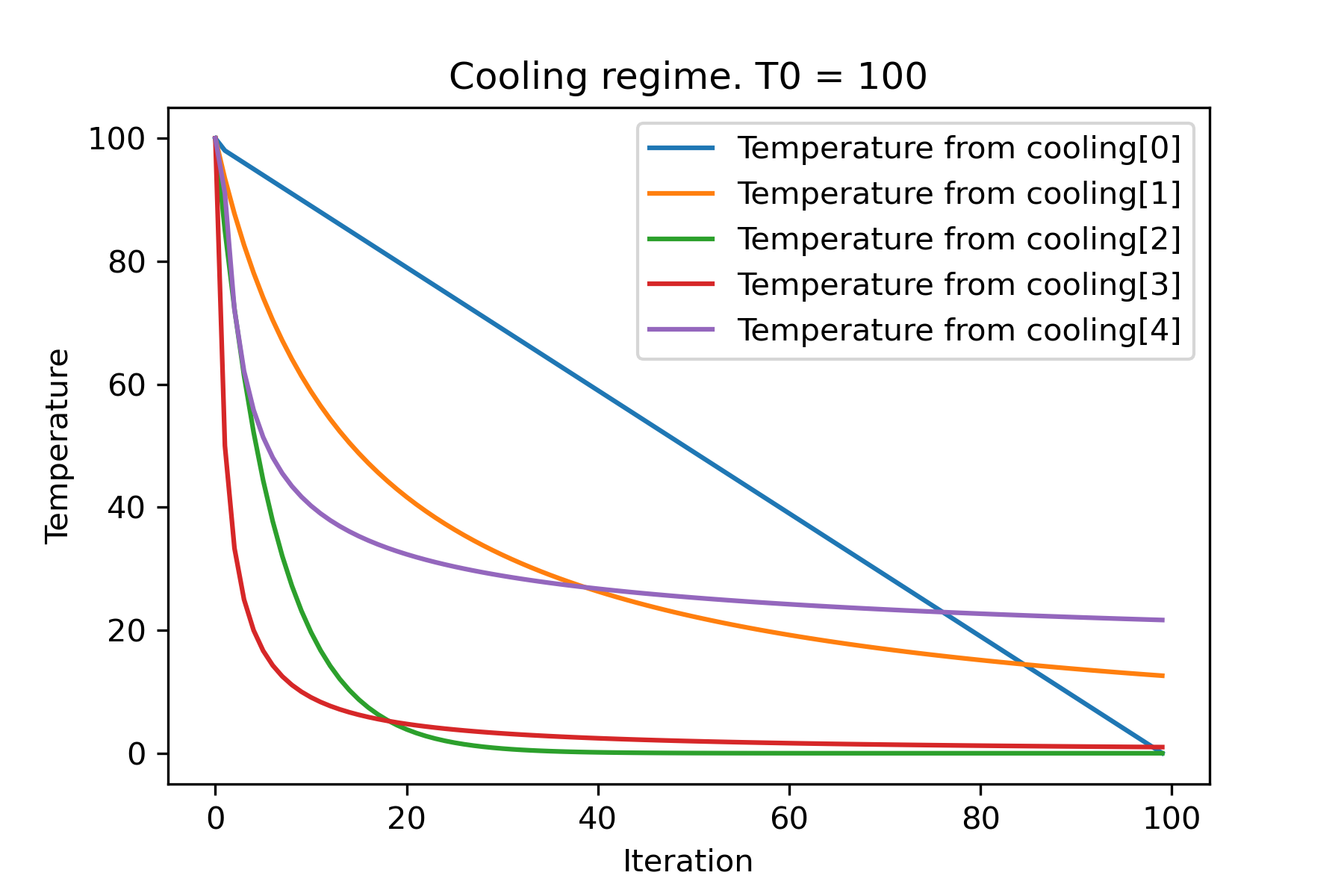
 # and we can set own temperature and cooling for each dimention!

temperature = [ 100 , 125 , 150 ]
cooling = [
    Cooling . exponential ( alpha = 0.85 ),
    Cooling . exponential ( alpha = 0.9 ),
    Cooling . exponential ( alpha = 0.95 ),
    ]
SimulatedAnnealing . plot_temperature ( cooling , temperature , iterations = 100 , save_as = 'diff_temp_and_cool.png' )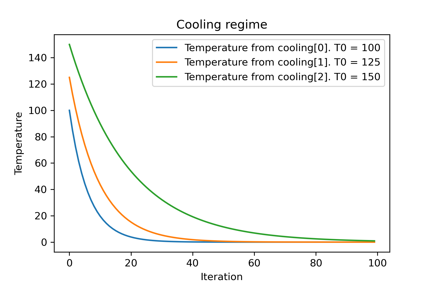
Por que existem tantos regimes de resfriamento? Para certa tarefa, um deles pode ser tão melhor! Neste script, podemos testar diferentes refrigeração para função de rasting:
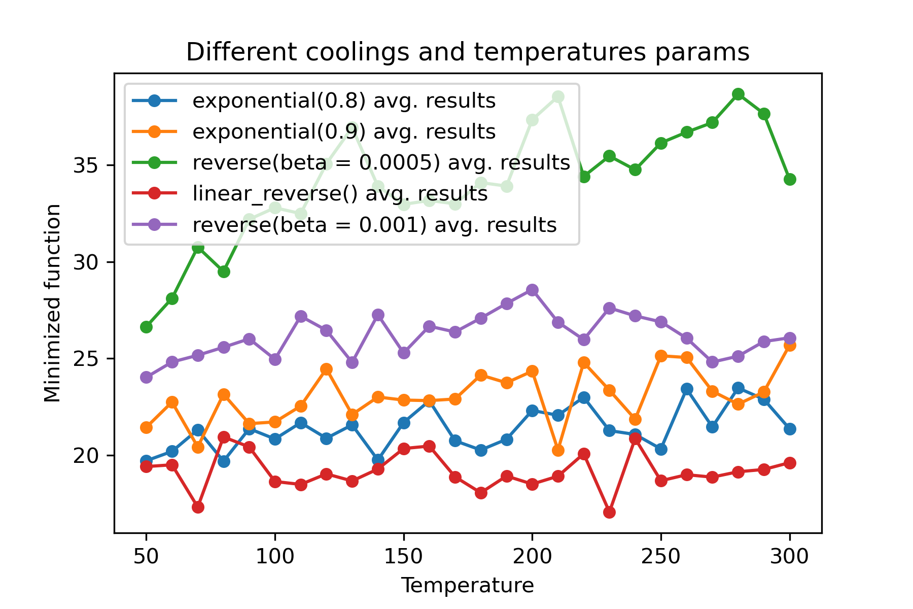
É uma característica incrível usar diferentes refrigerações e iniciar temperaturas para cada dimensão :
 import math
import numpy as np

from SimplestSimulatedAnnleaning import SimulatedAnnealing , Cooling , simple_continual_mutation


def Rastrigin ( arr ):
    return 10 * arr . size + np . sum ( arr ** 2 ) - 10 * np . sum ( np . cos ( 2 * math . pi * arr ))

dim = 5


model = SimulatedAnnealing ( Rastrigin , dim )

best_solution , best_val = model . run (
    start_solution = np . random . uniform ( - 5 , 5 , dim ),
    mutation = simple_continual_mutation ( std = 1 ),
    cooling = [ # different cooling for each dimention
        Cooling . exponential ( 0.8 ),
        Cooling . exponential ( 0.9 ),
        Cooling . reverse ( beta = 0.0005 ),
        Cooling . linear_reverse (),
        Cooling . reverse ( beta = 0.001 )
        ],
    start_temperature = 100 ,
    max_function_evals = 1000 ,
    max_iterations_without_progress = 250 ,
    step_for_reinit_temperature = 90 ,
    reinit_from_best = False
    )

print ( best_val )

model . plot_report ( save_as = 'different_coolings.png' )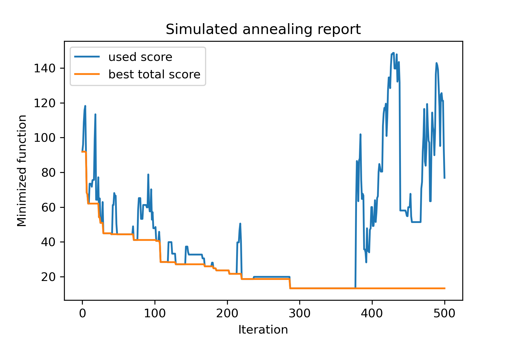
O principal motivo para usar vários refrigerantes é o comportamento específico de cada dimensão. Por exemplo, a primeira dimensão do espaço pode ser muito mais larga que a segunda dimensão, portanto, é melhor usar uma pesquisa mais ampla pela primeira dimensão; U pode produzi -lo usando a função mut especial, usando diferentes start temperatures e usando diferentes coolings .
Outro motivo para usar vários refrigerantes é o modo de seleção: para seleção de múltiplos refrigeros entre soluções boas e ruins, aplica -se por cada dimensão . Portanto, aumenta as chances de encontrar uma solução melhor.
A função de mutação é o parâmetro mais importante. Ele determina o comportamento da criação de novos objetos usando informações sobre o objeto atual e sobre a temperatura. Eu recomendo contar estes princípios ao criar a função mut :
Vamos lembrar da estrutura de mut :
 def mut ( x_as_array , temperature_as_array_or_one_number ):
    # some code
    return new_x_as_array
Aqui x_as_array é a solução atual e new_x_as_array é a solução mutada (aleatória e com o mesmo escuro, como você lembra). Você também deve se lembrar de que temperature_as_array_or_one_number é o número apenas para a solução não multifuncional. Caso contrário (ao usar várias temperaturas iniciais de vários resfriamentos ou ambos), é uma matriz Numpy . Veja exemplos
Neste exemplo, mostro como selecionar k objetos de Set com n objetos que minimizarão alguma função (neste exemplo: valor absoluto da mediana):
 import numpy as np
from SimplestSimulatedAnnleaning import SimulatedAnnealing , Cooling

SEED = 3

np . random . seed ( SEED )

Set = np . random . uniform ( low = - 15 , high = 5 , size = 100 ) # all set

dim = 10 # how many objects should we choose

indexes = np . arange ( Set . size )
# minimized function -- subset with best |median|
def min_func ( arr ):
    return abs ( np . median ( Set [ indexes [ arr . astype ( bool )]]))

# zero vectors with 'dim' ones at random positions
start_solution = np . zeros ( Set . size )
start_solution [ np . random . choice ( indexes , dim , replace = False )] = 1

# mutation function
# temperature is the number cuz we will use only 1 cooling, but it's not necessary to use it)
def mut ( x_as_array , temperature_as_array_or_one_number ):
    mask_one = x_as_array == 1
    mask_zero = np . logical_not ( mask_one )

    new_x_as_array = x_as_array . copy ()
    # replace some zeros with ones
    new_x_as_array [ np . random . choice ( indexes [ mask_one ], 1 , replace = False )] = 0
    new_x_as_array [ np . random . choice ( indexes [ mask_zero ], 1 , replace = False )] = 1

    return new_x_as_array

# creating a model
model = SimulatedAnnealing ( min_func , dim )

# run search
best_solution , best_val = model . run (
    start_solution = start_solution ,
    mutation = mut ,
    cooling = Cooling . exponential ( 0.9 ),
    start_temperature = 100 ,
    max_function_evals = 1000 ,
    max_iterations_without_progress = 100 ,
    step_for_reinit_temperature = 80 ,
    seed = SEED
    )

model . plot_report ( save_as = 'best_subset.png' )
Vamos dar uma olhada nesta tarefa:
 split set of values {v1, v2, v3, ..., vn} to sets 0, 1, 2, 3
with their sizes (volumes determined by user) to complete best sets metric
Uma das maneiras de resolvê -lo:
 from collections import defaultdict
import numpy as np

from SimplestSimulatedAnnleaning import SimulatedAnnealing , Cooling

################### useful methods

def counts_to_vec ( dic_count ):
    """
    converts dictionary like {1: 3, 2: 4}
    to array [1, 1, 1, 2, 2, 2, 2]
    """
    arrs = [ np . full ( val , fill_value = key ) for key , val in dic_count . items ()]

    return np . concatenate ( tuple ( arrs ))

def vec_to_indexes_dict ( vector ):
    """
    converts vector like [1, 0, 1, 2, 2]
    to dictionary with indexes {1: [0, 2], 2: [3, 4]}
    """

    res = defaultdict ( list )

    for i , v in enumerate ( vector ):
        res [ v ]. append ( i )

    return { int ( key ): np . array ( val ) for key , val in res . items () if key != 0 }


#################### START PARAMS

SEED = 3

np . random . seed ( SEED )

Set = np . random . uniform ( low = - 15 , high = 5 , size = 100 ) # all set
Set_indexes = np . arange ( Set . size )

# how many objects should be in each set
dim_dict = {
    1 : 10 ,
    2 : 10 ,
    3 : 7 ,
    4 : 14
}


# minimized function: sum of means vy each split set
def min_func ( arr ):

    indexes_dict = vec_to_indexes_dict ( arr )

    means = [ np . mean ( Set [ val ]) for val in indexes_dict . values ()]

    return sum ( means )

# zero vector with available set labels at random positions
start_solution = np . zeros ( Set . size , dtype = np . int8 )
labels_vec = counts_to_vec ( dim_dict )
start_solution [ np . random . choice ( Set_indexes , labels_vec . size , replace = False )] = labels_vec


def choice ( count = 3 ):
    return np . random . choice ( Set_indexes , count , replace = False )

# mutation function
# temperature is the number cuz we will use only 1 cooling, but it's not necessary to use it)
def mut ( x_as_array , temperature_as_array_or_one_number ):

    new_x_as_array = x_as_array . copy ()
    # replace some values

    while True :
        inds = choice ()

        if np . unique ( new_x_as_array [ inds ]). size == 1 : # there is no sense to replace same values
            continue
        new_x_as_array [ inds ] = new_x_as_array [ np . random . permutation ( inds )]

        return new_x_as_array

# creating a model
model = SimulatedAnnealing ( min_func , Set_indexes . size )

# run search
best_solution , best_val = model . run (
    start_solution = start_solution ,
    mutation = mut ,
    cooling = Cooling . exponential ( 0.9 ),
    start_temperature = 100 ,
    max_function_evals = 1000 ,
    max_iterations_without_progress = 100 ,
    step_for_reinit_temperature = 80 ,
    seed = SEED ,
    reinit_from_best = True
    )

model . plot_report ( save_as = 'best_split.png' )
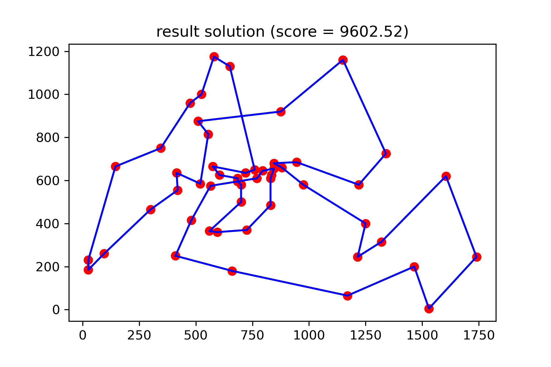
Vamos tentar resolver o problema do vendedor ambulante para a tarefa Berlin52. Nesta tarefa, existem 52 cidades com coordenadas do arquivo.
Em primeiro lugar, vamos importar pacotes:
 import math
import numpy as np
import pandas as pd
import matplotlib . pyplot as plt

from SimplestSimulatedAnnleaning import SimulatedAnnealing , Cooling
Defina semente para reprodução:
 SEED = 1
np . random . seed ( SEED )
Leia as coordenadas e crie matriz de distância:
 # read coordinates
coords = pd . read_csv ( 'berlin52_coords.txt' , sep = ' ' , header = None , names = [ 'index' , 'x' , 'y' ])

# dim is equal to count of cities
dim = coords . shape [ 0 ]

# distance matrix
distances = np . empty (( dim , dim ))

for i in range ( dim ):
    distances [ i , i ] = 0
    for j in range ( i + 1 , dim ):
        d = math . sqrt ( np . sum (( coords . iloc [ i , 1 :] - coords . iloc [ j , 1 :]) ** 2 ))
        distances [ i , j ] = d
        distances [ j , i ] = d
Crie solução de início aleatório:
 indexes = np . arange ( dim )
# some start solution (indexes shuffle)
start_solution = np . random . choice ( indexes , dim , replace = False )
Defina uma função que calcula a duração de passagem:
 # minized function
def way_length ( arr ):
    s = 0
    for i in range ( 1 , dim ):
        s += distances [ arr [ i - 1 ], arr [ i ]]
    # also we should end the way in the beggining
    s += distances [ arr [ - 1 ], arr [ 1 ]]

    return s
Vamos visualizar a solução inicial:
 def plotData ( indices , title , save_as = None ):

    # create a list of the corresponding city locations:
    locs = [ coords . iloc [ i , 1 :] for i in indices ]
    locs . append ( coords . iloc [ indices [ 0 ], 1 :])

    # plot a line between each pair of consequtive cities:
    plt . plot ( * zip ( * locs ), linestyle = '-' , color = 'blue' )

    # plot the dots representing the cities:
    plt . scatter ( coords . iloc [:, 1 ], coords . iloc [:, 2 ], marker = 'o' , s = 40 , color = 'red' )
    plt . title ( title )

    if not ( save_as is None ):  plt . savefig ( save_as , dpi = 300 )

    plt . show ()


# let's plot start solution
plotData ( start_solution , f'start random solution (score = { round ( way_length ( start_solution ), 2 ) } )' , 'salesman_start.png' )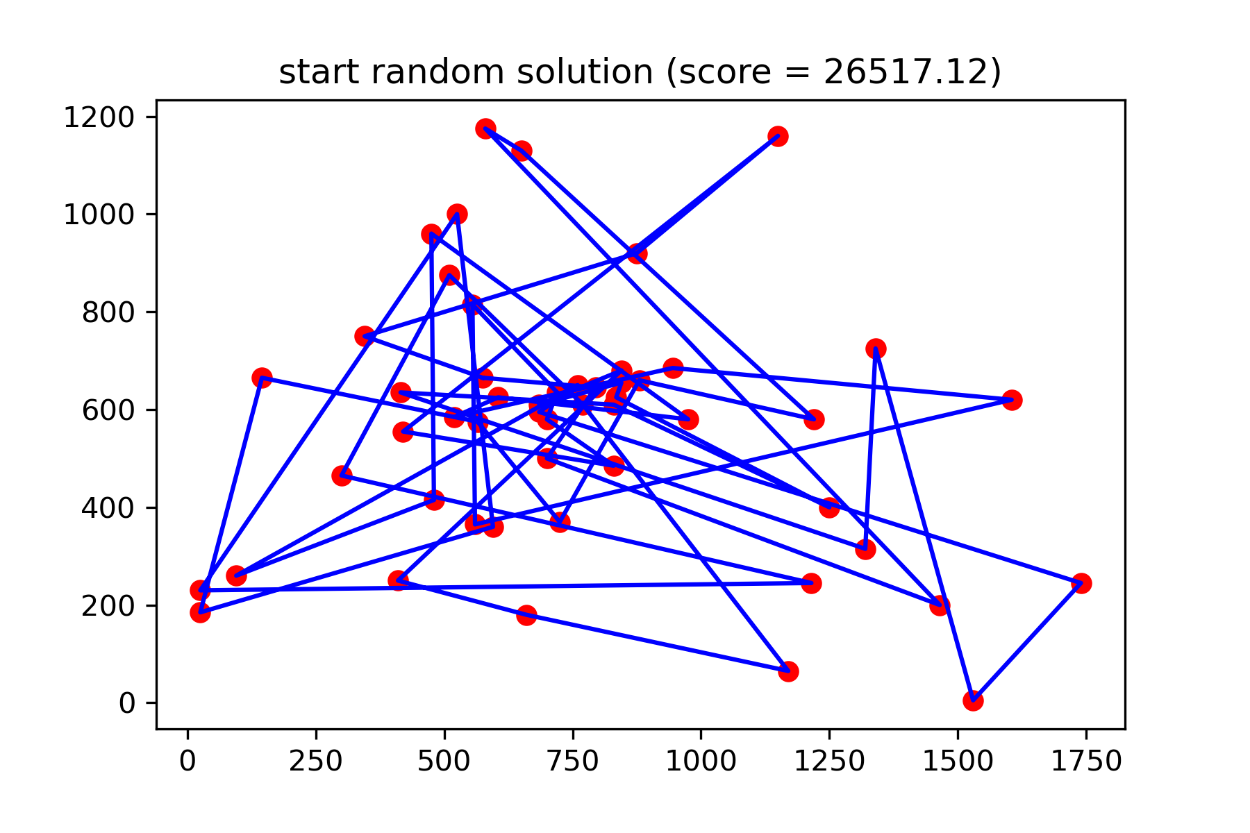
Realmente não é uma boa solução. Eu quero criar esta função de mutação para esta tarefa:
 def mut ( x_as_array , temperature_as_array_or_one_number ):
    # random indexes
    rand_inds = np . random . choice ( indexes , 3 , replace = False )
    # shuffled indexes
    goes_to = np . random . permutation ( rand_inds )

    # just replace some positions in the array
    new_x_as_array = x_as_array . copy ()
    new_x_as_array [ rand_inds ] = new_x_as_array [ goes_to ]

    return new_x_as_array
Comece a pesquisar:
 # creating a model
model = SimulatedAnnealing ( way_length , dim )

# run search
best_solution , best_val = model . run (
    start_solution = start_solution ,
    mutation = mut ,
    cooling = Cooling . exponential ( 0.9 ),
    start_temperature = 100 ,
    max_function_evals = 15000 ,
    max_iterations_without_progress = 2000 ,
    step_for_reinit_temperature = 80 ,
    reinit_from_best = True ,
    seed = SEED
    )

model . plot_report ( save_as = 'best_salesman.png' )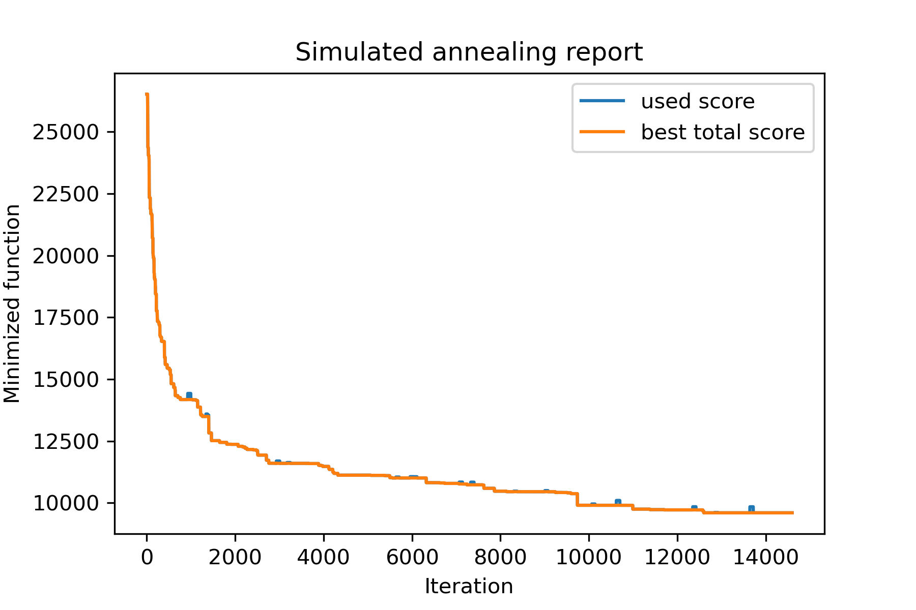
E veja nossa solução muito melhor:
plotData ( best_solution , f'result solution (score = { round ( best_val , 2 ) } )' , 'salesman_result.png' )