SimplestSimulatedAnnealing
1.0.0
Implementasi paling sederhana (dari DPEA) dari metode anil simulasi
pip install SimplestSimulatedAnnealing
Ini adalah algoritma evolusi untuk minimalisasi fungsi .
Tangga:
f harus diminimalkanx0 (bisa acak)mut . Fungsi ini harus memberikan solusi x1 yang baru (dapat acak) menggunakan informasi tentang x0 dan suhu T .cooling (perilaku suhu)Tx0 Solution dan f(x0) Skor Terbaikx1 = mut(x0) dan hitung f(x1)f(x1) < f(x0) , kami menemukan solusi yang lebih baik x0 = x1 . Kalau tidak, kita dapat mengganti x1 dengan x0 dengan probabilitas sama dengan exp((f(x0) - f(x1)) / T)T Menggunakan Fungsi cooling : T = cooling(T)Paket Impor:
 import math
import numpy as np

from SimplestSimulatedAnnleaning import SimulatedAnnealing , Cooling , simple_continual_mutation
Tentukan fungsi yang diminimalkan (rastrigin):
 def Rastrigin ( arr ):
    return 10 * arr . size + np . sum ( arr ** 2 ) - 10 * np . sum ( np . cos ( 2 * math . pi * arr ))

dim = 5
Kami akan menggunakan mutasi Gauss paling sederhana:
mut = simple_continual_mutation ( std = 0.5 )Buat objek model (set fungsi dan dimensi):
model = SimulatedAnnealing ( Rastrigin , dim )Mulailah mencari dan lihat laporan:
 best_solution , best_val = model . run (
    start_solution = np . random . uniform ( - 5 , 5 , dim ),
    mutation = mut ,
    cooling = Cooling . exponential ( 0.9 ),
    start_temperature = 100 ,
    max_function_evals = 1000 ,
    max_iterations_without_progress = 100 ,
    step_for_reinit_temperature = 80
    )

model . plot_report ( save_as = 'simple_example.png' )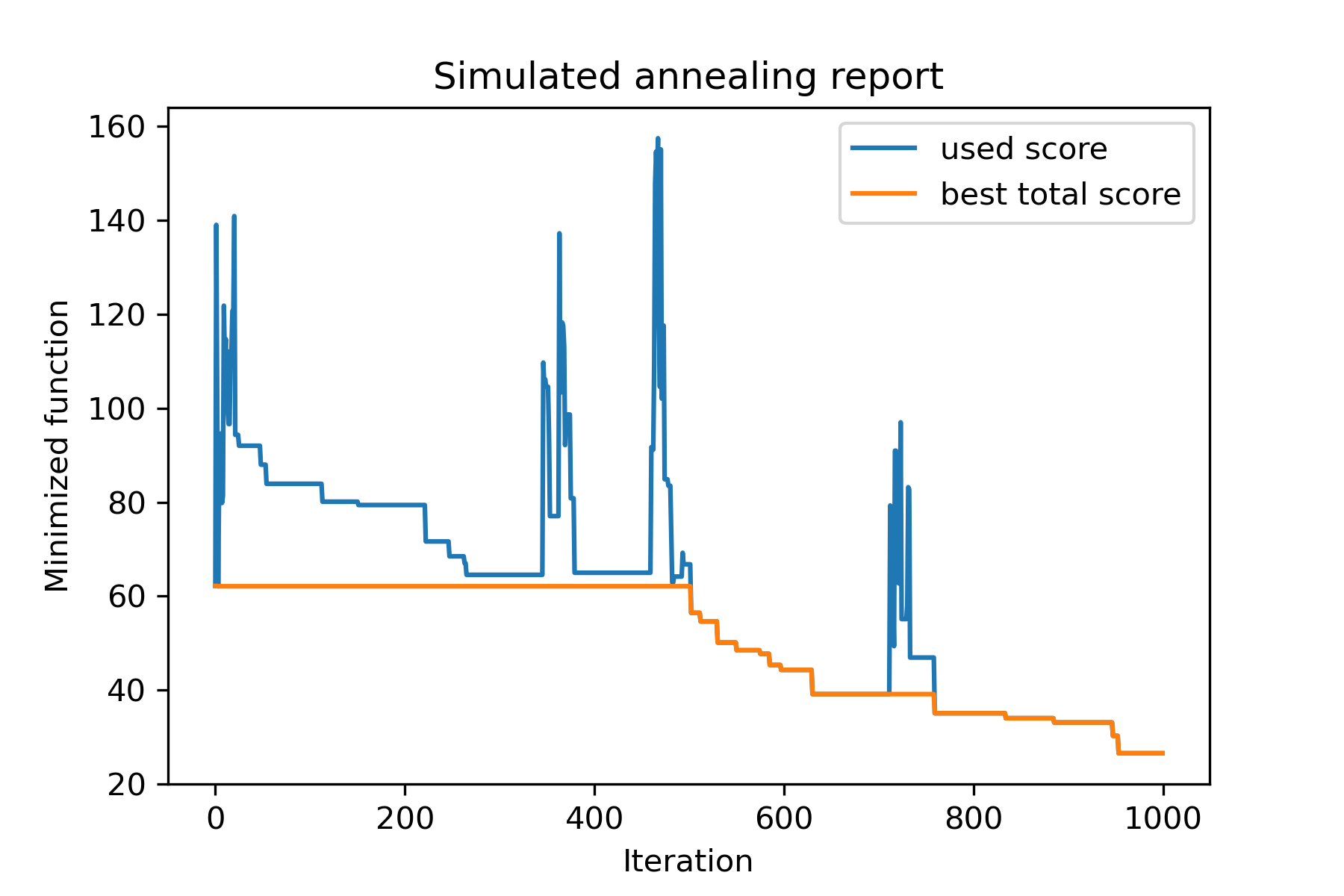
Metode utama paket adalah run() . Mari kita periksa argumennya:
 model . run ( start_solution ,
          mutation ,
          cooling ,
          start_temperature ,
          max_function_evals = 1000 ,
          max_iterations_without_progress = 250 ,
          step_for_reinit_temperature = 90 ,
          reinit_from_best = False ,
          seed = None )
Di mana:
start_solution : array numpy; solusi dari mana ia harus dimulai.
mutation : Fungsi (array, array/angka). Fungsi seperti
 def mut ( x_as_array , temperature_as_array_or_one_number ):
    # some code
    return new_x_as_array
Fungsi ini akan membuat solusi baru dari yang ada. Lihat juga
cooling : Daftar Fungsi / Fungsi Pendinginan. Fungsi pendinginan atau daftar yang. Melihat
start_temperature : Number atau nomor array (daftar/tuple). Mulai suhu. Dapat berupa satu angka atau array angka.
max_function_evals : int, opsional. Jumlah evaluasi fungsi maksimum. Standarnya adalah 1000.
max_iterations_without_progress : int, opsional. Jumlah iterasi maksimum tanpa kemajuan global. Standarnya adalah 250.
step_for_reinit_temperature : int, opsional. Setelah jumlah iterasi ini tanpa suhu kemajuan akan diinisialisasi seperti awal. Standarnya adalah 90.
reinit_from_best : boolean, opsional. Mulai algoritma dari solusi terbaik setelah suhu reinit (atau dari solusi terakhir saat ini). Standarnya false.
seed : int/none, opsional. Biji acak (jika perlu)
Bagian penting dari algoritma adalah fungsi pendinginan . Fungsi ini mengontrol nilai suhu tergantung pada angka iterasi saat ini, suhu arus dan suhu mulai. Anda dapat membuat fungsi pendingin Anda sendiri menggunakan pola:
 def func ( T_last , T0 , k ):
    # some code
    return T_new
Di sini T_last (int/float) adalah nilai suhu dari iterasi sebelumnya, T0 (int/float) adalah suhu awal dan k (int> 0) adalah jumlah iterasi. Anda harus menggunakan beberapa informasi ini untuk membuat suhu baru T_new .
Sangat disarankan untuk membangun fungsi Anda hanya untuk menciptakan suhu positif.
Di kelas Cooling ada beberapa fungsi pendingin:
Cooling.linear(mu, Tmin = 0.01)Cooling.exponential(alpha = 0.9)Cooling.reverse(beta = 0.0005)Cooling.logarithmic(c, d = 1) - tidak disarankanCooling.linear_reverse() Anda dapat melihat perilaku fungsi pendinginan menggunakan metode SimulatedAnnealing.plot_temperature . Mari kita lihat beberapa contoh:
 from SimplestSimulatedAnnleaning import SimulatedAnnealing , Cooling


# simplest way to set cooling regime
temperature = 100
cooling = Cooling . reverse ( beta = 0.001 )
# we can temperature behaviour using this code
SimulatedAnnealing . plot_temperature ( cooling , temperature , iterations = 100 , save_as = 'reverse.png' )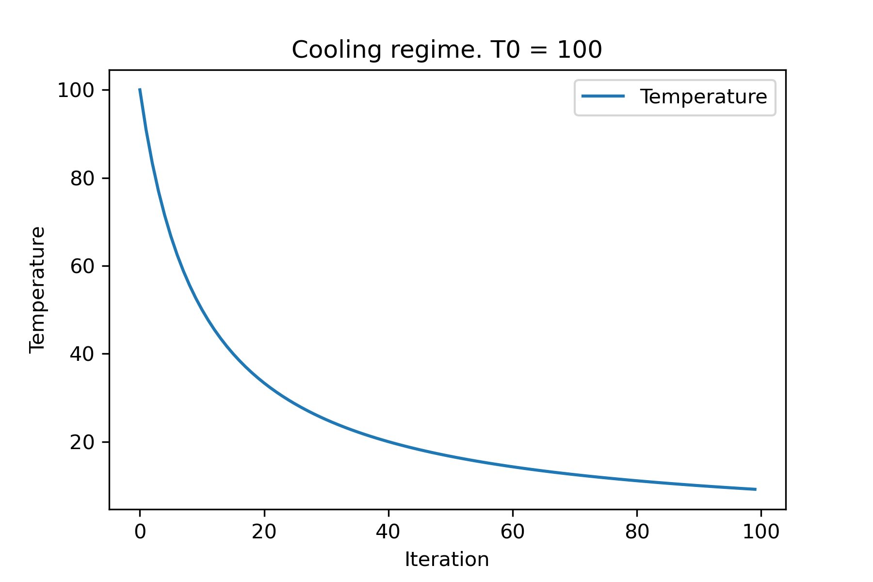
 # we can set several temparatures (for each dimention)
temperature = [ 150 , 100 , 50 ]
SimulatedAnnealing . plot_temperature ( cooling , temperature , iterations = 100 , save_as = 'reverse_diff_temp.png' )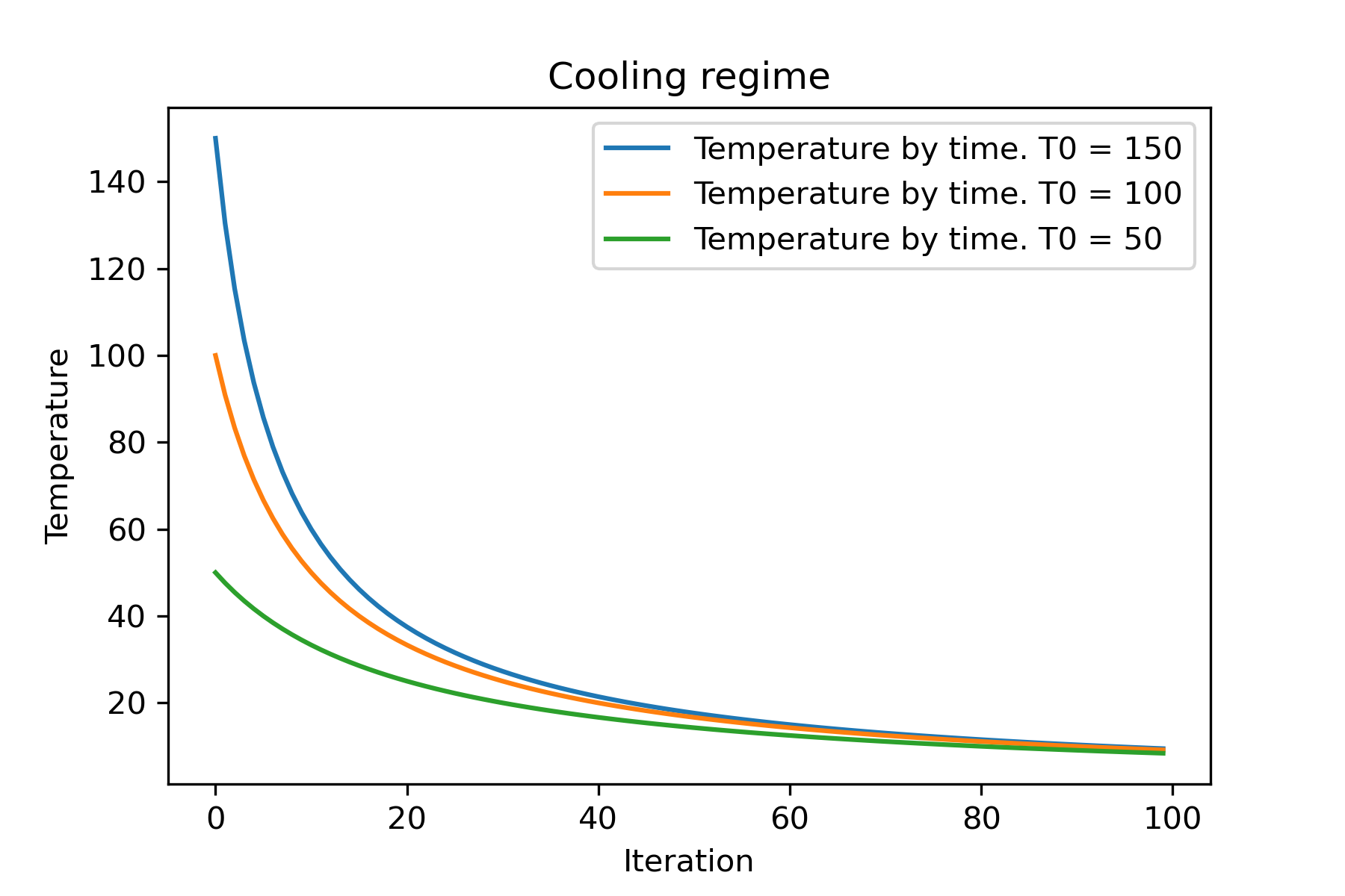
 # or several coolings (for each dimention)
temperature = 100
cooling = [
    Cooling . reverse ( beta = 0.0001 ),
    Cooling . reverse ( beta = 0.0005 ),
    Cooling . reverse ( beta = 0.001 )
    ]
SimulatedAnnealing . plot_temperature ( cooling , temperature , iterations = 100 , save_as = 'reverse_diff_beta.png' )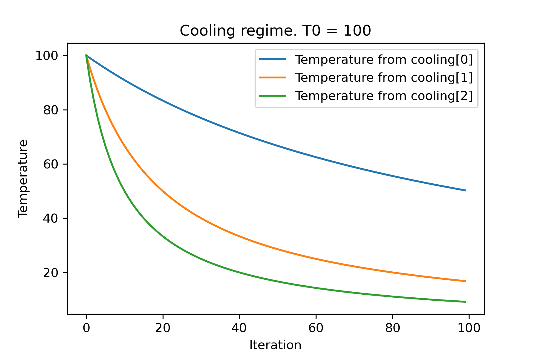
 # all supported coolling regimes

temperature = 100
cooling = [
    Cooling . linear ( mu = 1 ),
    Cooling . reverse ( beta = 0.0007 ),
    Cooling . exponential ( alpha = 0.85 ),
    Cooling . linear_reverse (),
    Cooling . logarithmic ( c = 100 , d = 1 )
    ]
SimulatedAnnealing . plot_temperature ( cooling , temperature , iterations = 100 , save_as = 'diff_temp.png' )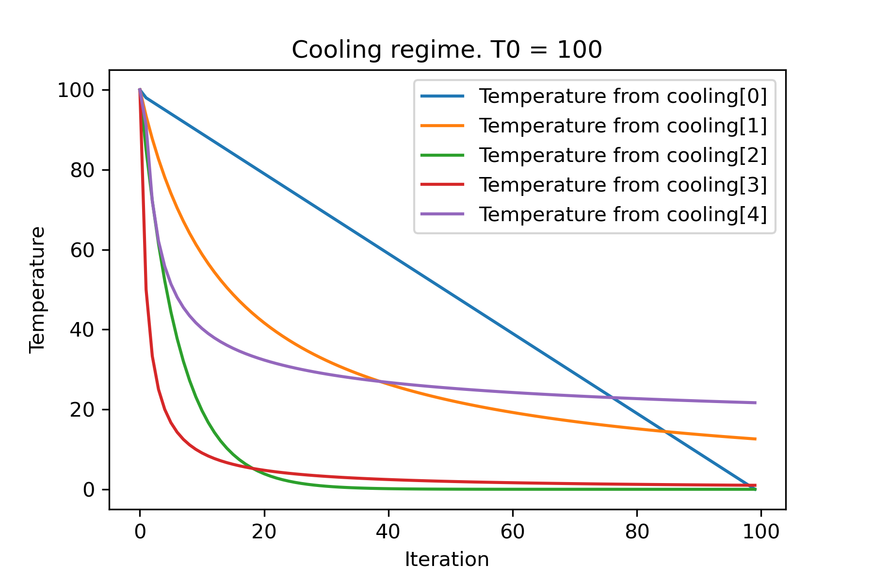
 # and we can set own temperature and cooling for each dimention!

temperature = [ 100 , 125 , 150 ]
cooling = [
    Cooling . exponential ( alpha = 0.85 ),
    Cooling . exponential ( alpha = 0.9 ),
    Cooling . exponential ( alpha = 0.95 ),
    ]
SimulatedAnnealing . plot_temperature ( cooling , temperature , iterations = 100 , save_as = 'diff_temp_and_cool.png' )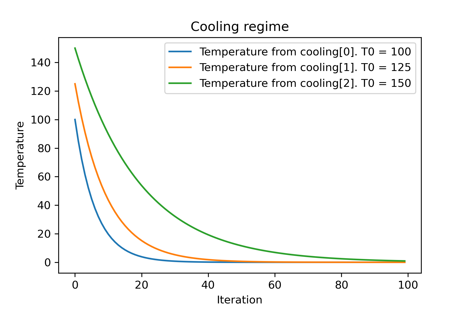
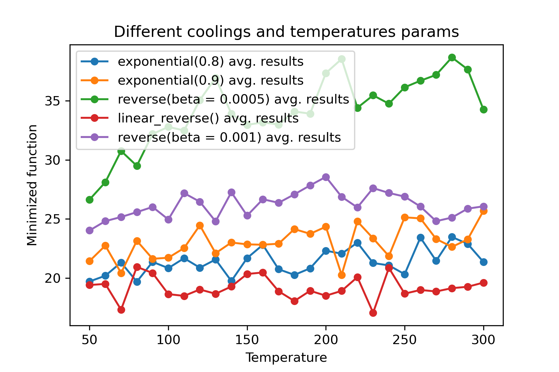
Mengapa ada begitu banyak rezim pendingin? Untuk tugas tertentu, salah satunya bisa menjadi lebih baik! Dalam skrip ini kita dapat menguji pendinginan yang berbeda untuk fungsi rastring:
Ini fitur yang luar biasa untuk menggunakan pendinginan yang berbeda dan memulai suhu untuk setiap dimensi :
 import math
import numpy as np

from SimplestSimulatedAnnleaning import SimulatedAnnealing , Cooling , simple_continual_mutation


def Rastrigin ( arr ):
    return 10 * arr . size + np . sum ( arr ** 2 ) - 10 * np . sum ( np . cos ( 2 * math . pi * arr ))

dim = 5


model = SimulatedAnnealing ( Rastrigin , dim )

best_solution , best_val = model . run (
    start_solution = np . random . uniform ( - 5 , 5 , dim ),
    mutation = simple_continual_mutation ( std = 1 ),
    cooling = [ # different cooling for each dimention
        Cooling . exponential ( 0.8 ),
        Cooling . exponential ( 0.9 ),
        Cooling . reverse ( beta = 0.0005 ),
        Cooling . linear_reverse (),
        Cooling . reverse ( beta = 0.001 )
        ],
    start_temperature = 100 ,
    max_function_evals = 1000 ,
    max_iterations_without_progress = 250 ,
    step_for_reinit_temperature = 90 ,
    reinit_from_best = False
    )

print ( best_val )

model . plot_report ( save_as = 'different_coolings.png' )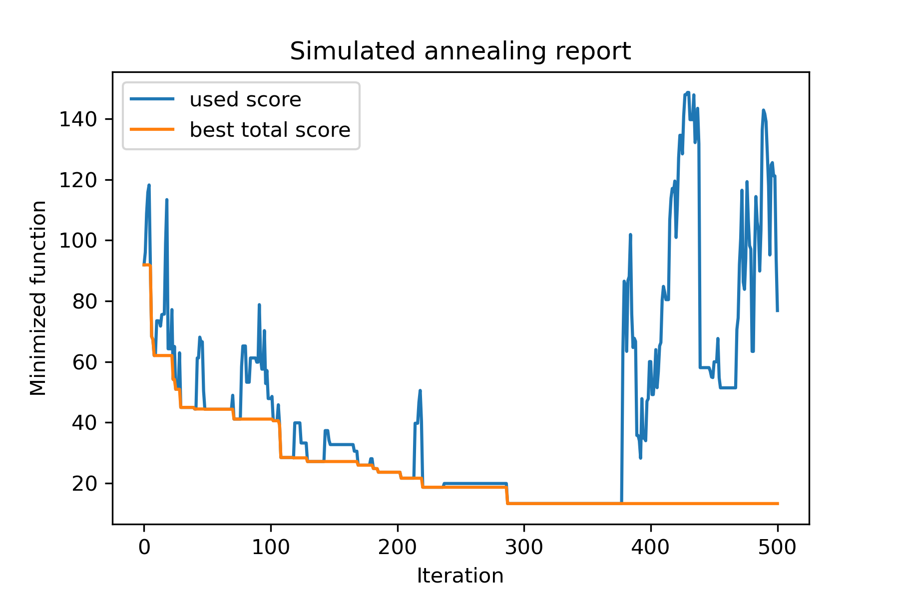
Alasan utama untuk menggunakan beberapa pendinginan adalah perilaku menentukan dari setiap dimensi. Misalnya, dimensi ruang pertama bisa jauh lebih luas dari dimensi kedua karena itu lebih baik menggunakan pencarian yang lebih luas untuk dimensi pertama; Anda dapat memproduksinya menggunakan fungsi mut khusus, menggunakan start temperatures yang berbeda dan menggunakan coolings yang berbeda.
Alasan lain untuk menggunakan beberapa pendinginan adalah cara seleksi: untuk beberapa pemilihan pendingin antara solusi baik dan buruk berlaku oleh setiap dimensi . Jadi, itu meningkatkan peluang untuk menemukan solusi yang lebih baik.
Fungsi mutasi adalah parameter terpenting. Ini menentukan perilaku membuat objek baru menggunakan informasi tentang objek saat ini dan tentang suhu. Saya merekomendasikan untuk menghitung prinsip -prinsip ini saat membuat fungsi mut :
Mari kita ingat struktur mut :
 def mut ( x_as_array , temperature_as_array_or_one_number ):
    # some code
    return new_x_as_array
Di sini x_as_array adalah solusi saat ini dan new_x_as_array adalah solusi bermutasi (acak dan dengan redup yang sama, seperti yang Anda ingat). Anda juga harus ingat bahwa temperature_as_array_or_one_number hanya nomor untuk solusi non-multicooling. Kalau tidak (saat menggunakan beberapa suhu mulai dari beberapa pendinginan atau keduanya) itu adalah array yang tidak bagus . Lihat contoh
Dalam contoh ini saya menunjukkan cara memilih objek k dari set dengan n objek yang akan meminimalkan beberapa fungsi (dalam contoh ini: nilai absolut median):
 import numpy as np
from SimplestSimulatedAnnleaning import SimulatedAnnealing , Cooling

SEED = 3

np . random . seed ( SEED )

Set = np . random . uniform ( low = - 15 , high = 5 , size = 100 ) # all set

dim = 10 # how many objects should we choose

indexes = np . arange ( Set . size )
# minimized function -- subset with best |median|
def min_func ( arr ):
    return abs ( np . median ( Set [ indexes [ arr . astype ( bool )]]))

# zero vectors with 'dim' ones at random positions
start_solution = np . zeros ( Set . size )
start_solution [ np . random . choice ( indexes , dim , replace = False )] = 1

# mutation function
# temperature is the number cuz we will use only 1 cooling, but it's not necessary to use it)
def mut ( x_as_array , temperature_as_array_or_one_number ):
    mask_one = x_as_array == 1
    mask_zero = np . logical_not ( mask_one )

    new_x_as_array = x_as_array . copy ()
    # replace some zeros with ones
    new_x_as_array [ np . random . choice ( indexes [ mask_one ], 1 , replace = False )] = 0
    new_x_as_array [ np . random . choice ( indexes [ mask_zero ], 1 , replace = False )] = 1

    return new_x_as_array

# creating a model
model = SimulatedAnnealing ( min_func , dim )

# run search
best_solution , best_val = model . run (
    start_solution = start_solution ,
    mutation = mut ,
    cooling = Cooling . exponential ( 0.9 ),
    start_temperature = 100 ,
    max_function_evals = 1000 ,
    max_iterations_without_progress = 100 ,
    step_for_reinit_temperature = 80 ,
    seed = SEED
    )

model . plot_report ( save_as = 'best_subset.png' )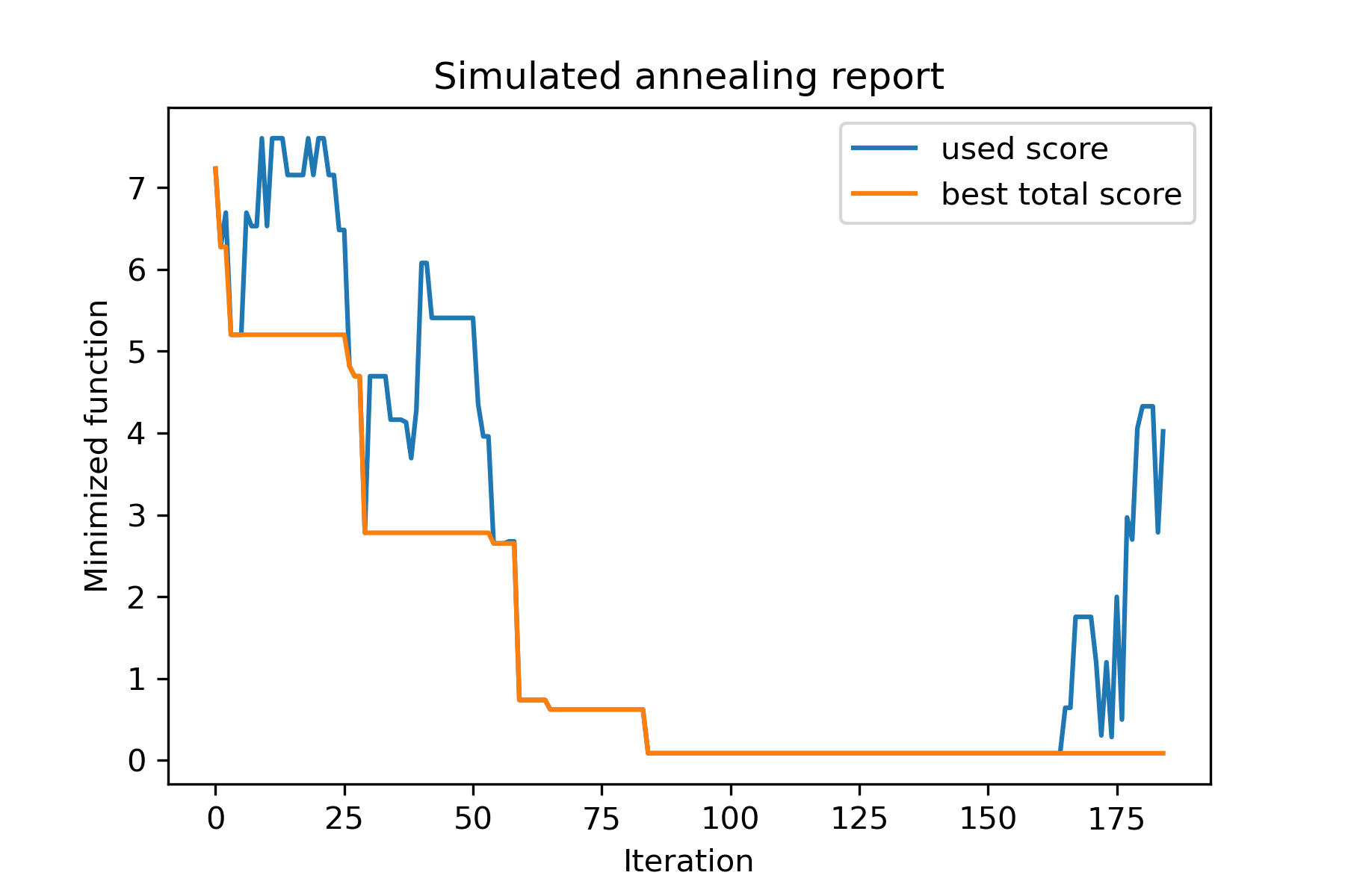
Mari kita lihat tugas ini:
 split set of values {v1, v2, v3, ..., vn} to sets 0, 1, 2, 3
with their sizes (volumes determined by user) to complete best sets metric
Salah satu cara untuk menyelesaikannya:
 from collections import defaultdict
import numpy as np

from SimplestSimulatedAnnleaning import SimulatedAnnealing , Cooling

################### useful methods

def counts_to_vec ( dic_count ):
    """
    converts dictionary like {1: 3, 2: 4}
    to array [1, 1, 1, 2, 2, 2, 2]
    """
    arrs = [ np . full ( val , fill_value = key ) for key , val in dic_count . items ()]

    return np . concatenate ( tuple ( arrs ))

def vec_to_indexes_dict ( vector ):
    """
    converts vector like [1, 0, 1, 2, 2]
    to dictionary with indexes {1: [0, 2], 2: [3, 4]}
    """

    res = defaultdict ( list )

    for i , v in enumerate ( vector ):
        res [ v ]. append ( i )

    return { int ( key ): np . array ( val ) for key , val in res . items () if key != 0 }


#################### START PARAMS

SEED = 3

np . random . seed ( SEED )

Set = np . random . uniform ( low = - 15 , high = 5 , size = 100 ) # all set
Set_indexes = np . arange ( Set . size )

# how many objects should be in each set
dim_dict = {
    1 : 10 ,
    2 : 10 ,
    3 : 7 ,
    4 : 14
}


# minimized function: sum of means vy each split set
def min_func ( arr ):

    indexes_dict = vec_to_indexes_dict ( arr )

    means = [ np . mean ( Set [ val ]) for val in indexes_dict . values ()]

    return sum ( means )

# zero vector with available set labels at random positions
start_solution = np . zeros ( Set . size , dtype = np . int8 )
labels_vec = counts_to_vec ( dim_dict )
start_solution [ np . random . choice ( Set_indexes , labels_vec . size , replace = False )] = labels_vec


def choice ( count = 3 ):
    return np . random . choice ( Set_indexes , count , replace = False )

# mutation function
# temperature is the number cuz we will use only 1 cooling, but it's not necessary to use it)
def mut ( x_as_array , temperature_as_array_or_one_number ):

    new_x_as_array = x_as_array . copy ()
    # replace some values

    while True :
        inds = choice ()

        if np . unique ( new_x_as_array [ inds ]). size == 1 : # there is no sense to replace same values
            continue
        new_x_as_array [ inds ] = new_x_as_array [ np . random . permutation ( inds )]

        return new_x_as_array

# creating a model
model = SimulatedAnnealing ( min_func , Set_indexes . size )

# run search
best_solution , best_val = model . run (
    start_solution = start_solution ,
    mutation = mut ,
    cooling = Cooling . exponential ( 0.9 ),
    start_temperature = 100 ,
    max_function_evals = 1000 ,
    max_iterations_without_progress = 100 ,
    step_for_reinit_temperature = 80 ,
    seed = SEED ,
    reinit_from_best = True
    )

model . plot_report ( save_as = 'best_split.png' )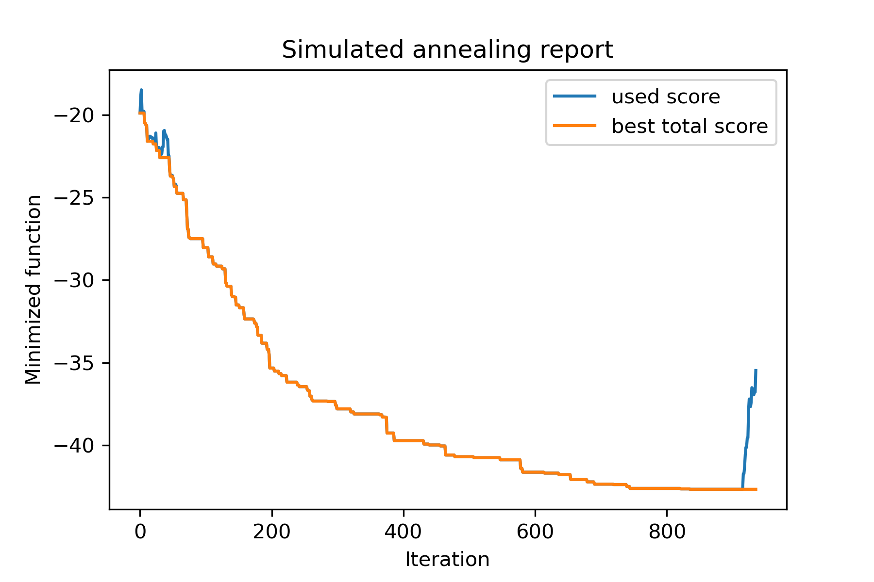
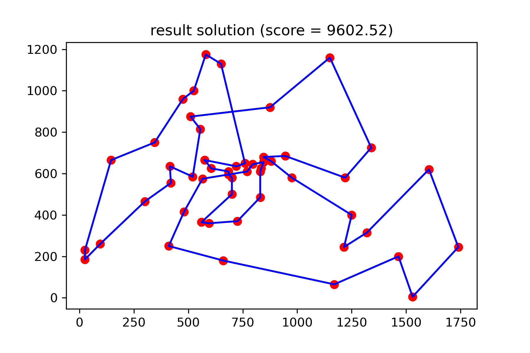
Mari kita coba menyelesaikan masalah salesman keliling untuk tugas Berlin52. Dalam tugas ini ada 52 kota dengan koordinat dari file.
Pertama, mari kita impor paket:
 import math
import numpy as np
import pandas as pd
import matplotlib . pyplot as plt

from SimplestSimulatedAnnleaning import SimulatedAnnealing , Cooling
Atur Seed untuk mereproduksi:
 SEED = 1
np . random . seed ( SEED )
Baca koordinat dan buat matriks jarak:
 # read coordinates
coords = pd . read_csv ( 'berlin52_coords.txt' , sep = ' ' , header = None , names = [ 'index' , 'x' , 'y' ])

# dim is equal to count of cities
dim = coords . shape [ 0 ]

# distance matrix
distances = np . empty (( dim , dim ))

for i in range ( dim ):
    distances [ i , i ] = 0
    for j in range ( i + 1 , dim ):
        d = math . sqrt ( np . sum (( coords . iloc [ i , 1 :] - coords . iloc [ j , 1 :]) ** 2 ))
        distances [ i , j ] = d
        distances [ j , i ] = d
Buat solusi start acak:
 indexes = np . arange ( dim )
# some start solution (indexes shuffle)
start_solution = np . random . choice ( indexes , dim , replace = False )
Tentukan fungsi yang menghitung panjang jalan:
 # minized function
def way_length ( arr ):
    s = 0
    for i in range ( 1 , dim ):
        s += distances [ arr [ i - 1 ], arr [ i ]]
    # also we should end the way in the beggining
    s += distances [ arr [ - 1 ], arr [ 1 ]]

    return s
Mari kita visualisasikan solusi mulai:
 def plotData ( indices , title , save_as = None ):

    # create a list of the corresponding city locations:
    locs = [ coords . iloc [ i , 1 :] for i in indices ]
    locs . append ( coords . iloc [ indices [ 0 ], 1 :])

    # plot a line between each pair of consequtive cities:
    plt . plot ( * zip ( * locs ), linestyle = '-' , color = 'blue' )

    # plot the dots representing the cities:
    plt . scatter ( coords . iloc [:, 1 ], coords . iloc [:, 2 ], marker = 'o' , s = 40 , color = 'red' )
    plt . title ( title )

    if not ( save_as is None ):  plt . savefig ( save_as , dpi = 300 )

    plt . show ()


# let's plot start solution
plotData ( start_solution , f'start random solution (score = { round ( way_length ( start_solution ), 2 ) } )' , 'salesman_start.png' )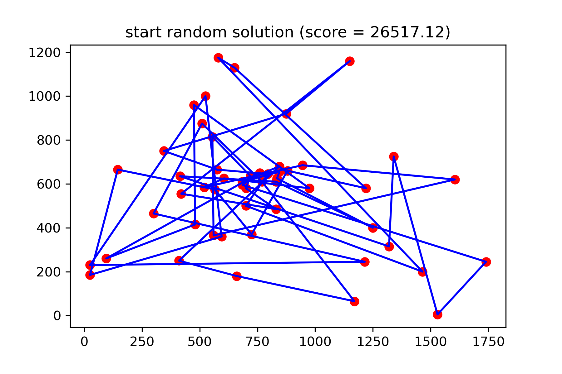
Ini benar -benar solusi yang tidak bagus. Saya ingin membuat fungsi mutasi ini untuk tugas ini:
 def mut ( x_as_array , temperature_as_array_or_one_number ):
    # random indexes
    rand_inds = np . random . choice ( indexes , 3 , replace = False )
    # shuffled indexes
    goes_to = np . random . permutation ( rand_inds )

    # just replace some positions in the array
    new_x_as_array = x_as_array . copy ()
    new_x_as_array [ rand_inds ] = new_x_as_array [ goes_to ]

    return new_x_as_array
Mulailah mencari:
 # creating a model
model = SimulatedAnnealing ( way_length , dim )

# run search
best_solution , best_val = model . run (
    start_solution = start_solution ,
    mutation = mut ,
    cooling = Cooling . exponential ( 0.9 ),
    start_temperature = 100 ,
    max_function_evals = 15000 ,
    max_iterations_without_progress = 2000 ,
    step_for_reinit_temperature = 80 ,
    reinit_from_best = True ,
    seed = SEED
    )

model . plot_report ( save_as = 'best_salesman.png' )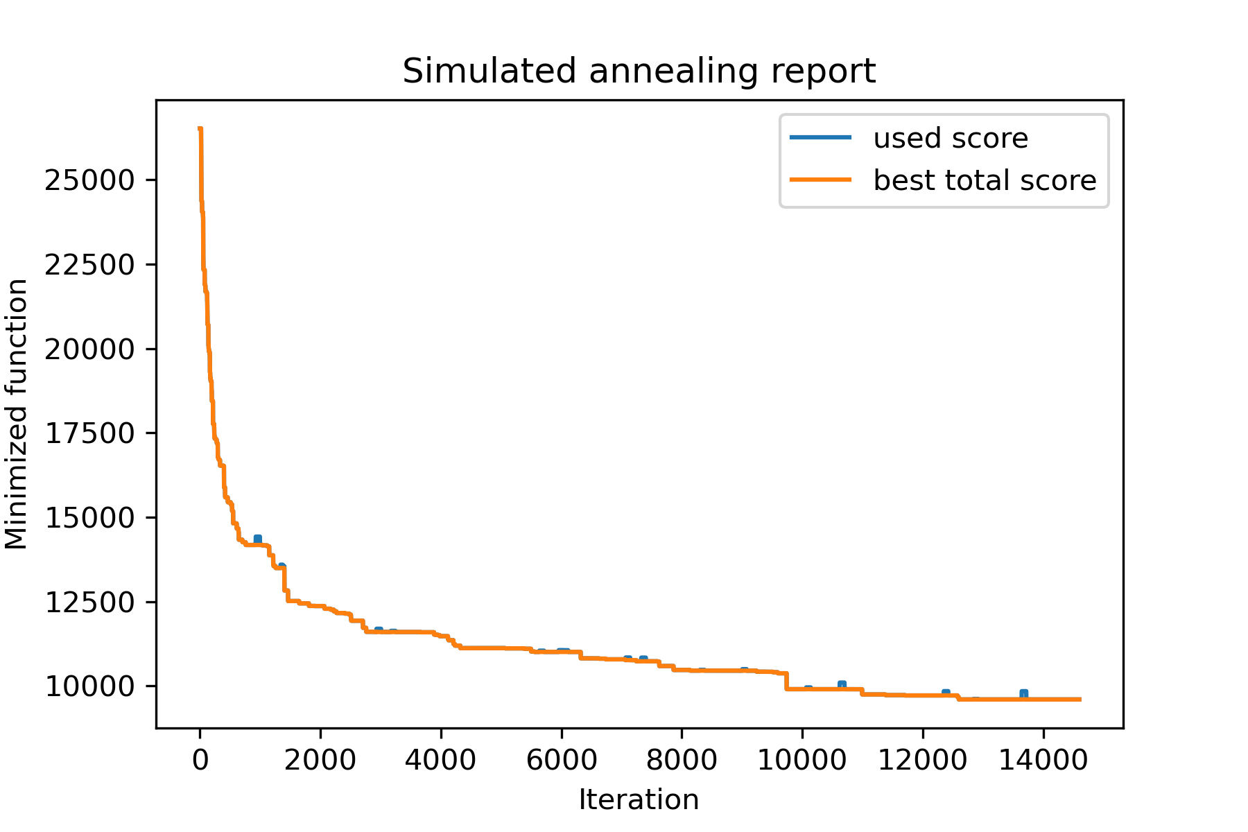
Dan lihat solusi kami yang jauh lebih baik:
plotData ( best_solution , f'result solution (score = { round ( best_val , 2 ) } )' , 'salesman_result.png' )