SimplestSimulatedAnnealing
1.0.0
シミュレートされたアニーリング法の最も単純な実装(DPEAから)
pip install SimplestSimulatedAnnealing
これは、関数最小化のための進化的アルゴリズムです。
ステップ:
fを最小化する必要があると判断する必要がありますx0を決定する(ランダムになる可能性があります)mutを決定します。この関数は、 x0と温度Tに関する情報を使用して、新しい(ランダムになる可能性がある) x1ソリューションを提供する必要があります。cooling体制(温度の動作)を選択または作成するTを設定しますx0ソリューションとf(x0)ベストスコアを持っていますx1 = mut(x0)を作成し、 f(x1)を計算しましょうf(x1) < f(x0)の場合、より良いソリューションx0 = x1見つかりました。それ以外の場合は、 x1 x0で確率で置き換えることができますexp((f(x0) - f(x1)) / T)cooling機能を使用してTを減らす: T = cooling(T)インポートパッケージ:
 import math
import numpy as np

from SimplestSimulatedAnnleaning import SimulatedAnnealing , Cooling , simple_continual_mutation
最小化関数を決定する(rastrigin):
 def Rastrigin ( arr ):
    return 10 * arr . size + np . sum ( arr ** 2 ) - 10 * np . sum ( np . cos ( 2 * math . pi * arr ))

dim = 5
最も単純なガウス変異を使用します:
mut = simple_continual_mutation ( std = 0.5 )モデルオブジェクトを作成します(機能と寸法を設定):
model = SimulatedAnnealing ( Rastrigin , dim )検索を開始してレポートを参照してください:
 best_solution , best_val = model . run (
    start_solution = np . random . uniform ( - 5 , 5 , dim ),
    mutation = mut ,
    cooling = Cooling . exponential ( 0.9 ),
    start_temperature = 100 ,
    max_function_evals = 1000 ,
    max_iterations_without_progress = 100 ,
    step_for_reinit_temperature = 80
    )

model . plot_report ( save_as = 'simple_example.png' )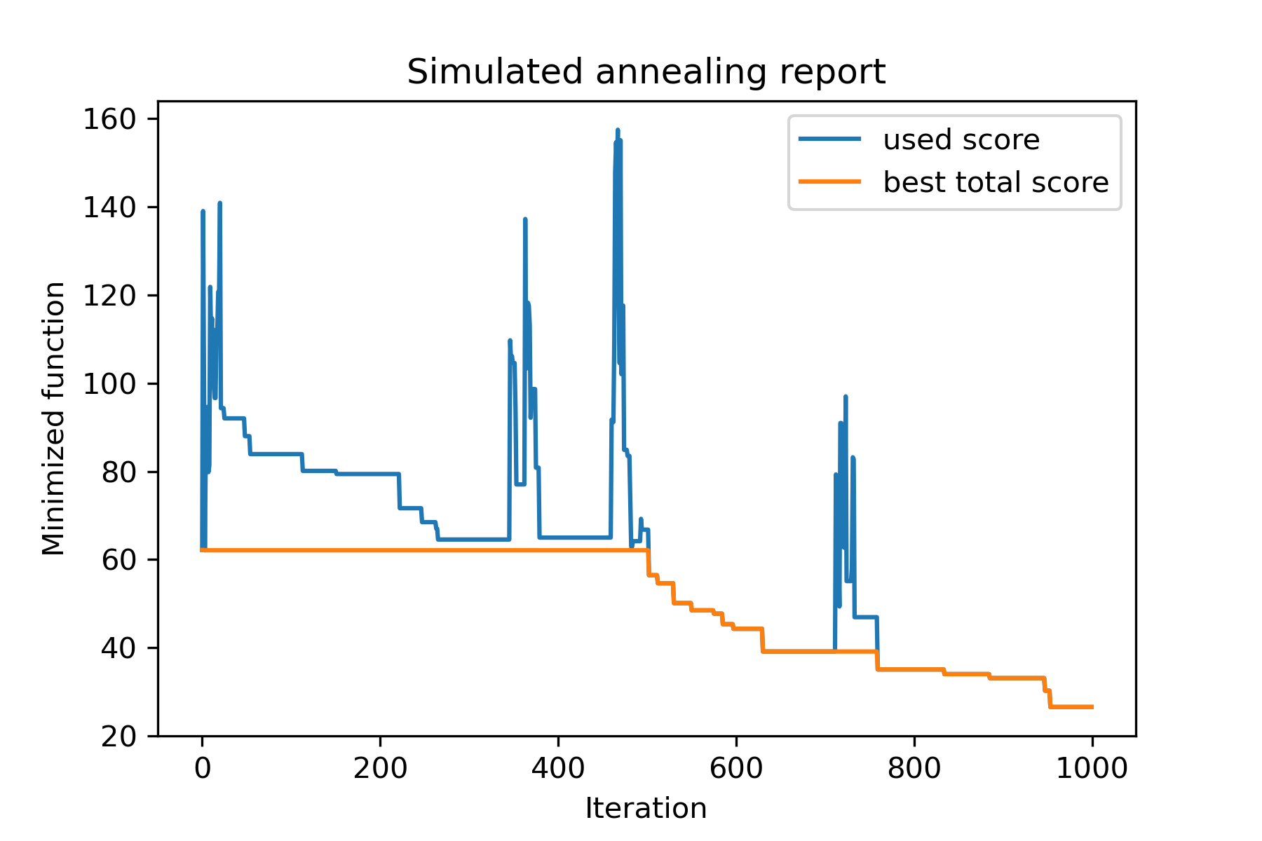
パッケージの主な方法はrun() 。それが議論であることを確認しましょう:
 model . run ( start_solution ,
          mutation ,
          cooling ,
          start_temperature ,
          max_function_evals = 1000 ,
          max_iterations_without_progress = 250 ,
          step_for_reinit_temperature = 90 ,
          reinit_from_best = False ,
          seed = None )
どこ:
start_solution :numpy配列;起動する解決策。
mutation :関数(配列、配列/番号)。のような機能
 def mut ( x_as_array , temperature_as_array_or_one_number ):
    # some code
    return new_x_as_array
この関数は、既存の新しいソリューションを作成します。参照してください
cooling :冷却機能 /関数リスト。冷却機能またはリストのリスト。見る
start_temperature :number or number array(list/tuple)。温度を開始します。 1つまたは数字の配列にすることができます。
max_function_evals :int、optional。関数評価の最大数。デフォルトは1000です。
max_iterations_without_progress :int、optional。グローバルな進歩のない最大反復数。デフォルトは250です。
step_for_reinit_temperature :int、optional。進行状況のないこの数の反復後、温度は開始のように初期化されます。デフォルトは90です。
reinit_from_best :boolean、オプション。温度を再度再生した後(または最後の電流溶液から)ベストソリューションからアルゴリズムを開始します。デフォルトはfalseです。
seed :int/none、オプション。ランダムシード(必要に応じて)
アルゴリズムの重要な部分は冷却機能です。この関数は、電流反復数、電流温度、および開始温度に依存する温度値を制御します。 Uは、パターンを使用して独自の冷却機能を作成できます。
 def func ( T_last , T0 , k ):
    # some code
    return T_new
ここでは、 T_last (int/float)は以前の反復からの温度値、 T0 (int/float)は開始温度、 k (int> 0)は反復数です。この情報の一部を使用して、新しい温度T_new作成する必要があります。
正の温度のみを作成するために機能を構築することを強くお勧めします。
Coolingクラスには、いくつかの冷却機能があります。
Cooling.linear(mu, Tmin = 0.01)Cooling.exponential(alpha = 0.9)Cooling.reverse(beta = 0.0005)Cooling.logarithmic(c, d = 1) - 推奨されませんCooling.linear_reverse()uは、 SimulatedAnnealing.plot_temperatureメソッドを使用して、冷却機能の動作を見ることができます。いくつかの例を見てみましょう:
 from SimplestSimulatedAnnleaning import SimulatedAnnealing , Cooling


# simplest way to set cooling regime
temperature = 100
cooling = Cooling . reverse ( beta = 0.001 )
# we can temperature behaviour using this code
SimulatedAnnealing . plot_temperature ( cooling , temperature , iterations = 100 , save_as = 'reverse.png' )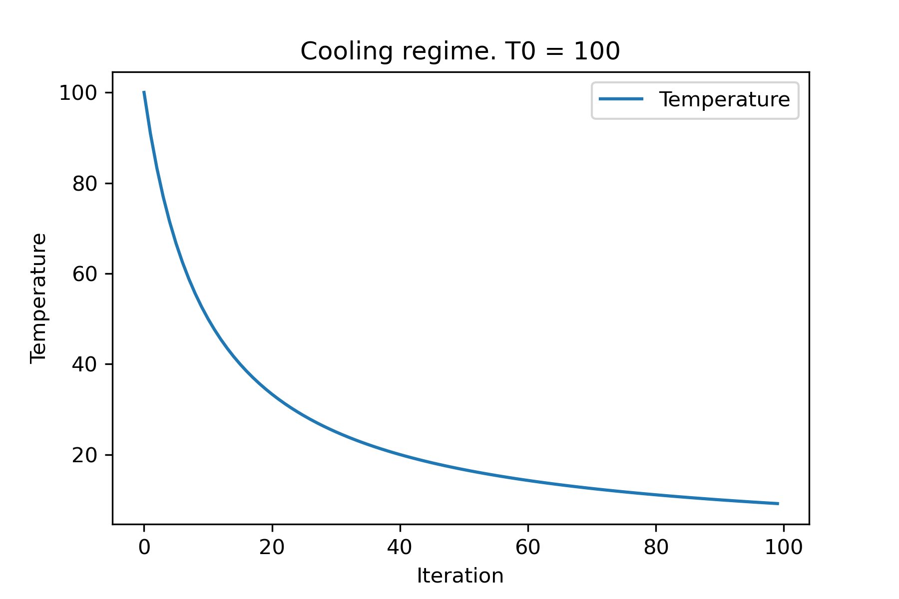
 # we can set several temparatures (for each dimention)
temperature = [ 150 , 100 , 50 ]
SimulatedAnnealing . plot_temperature ( cooling , temperature , iterations = 100 , save_as = 'reverse_diff_temp.png' )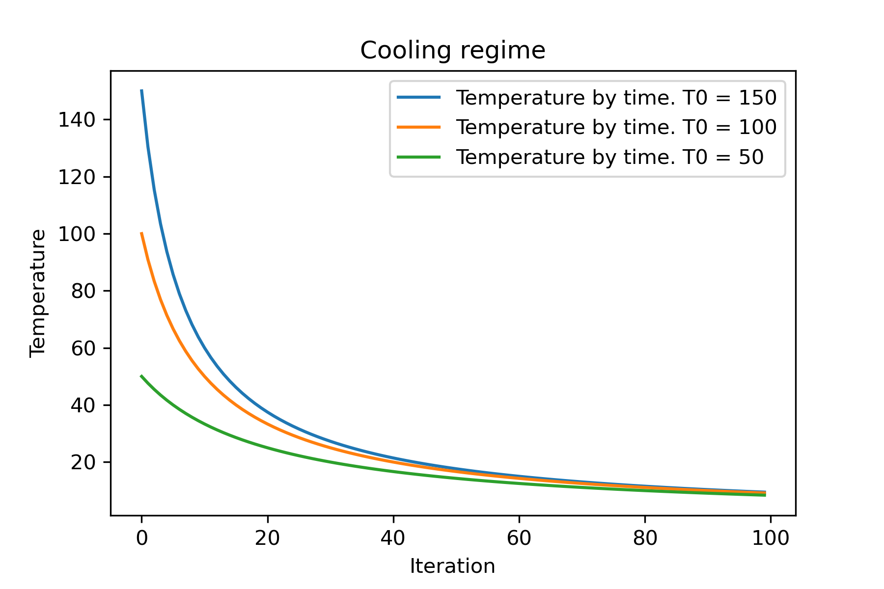
 # or several coolings (for each dimention)
temperature = 100
cooling = [
    Cooling . reverse ( beta = 0.0001 ),
    Cooling . reverse ( beta = 0.0005 ),
    Cooling . reverse ( beta = 0.001 )
    ]
SimulatedAnnealing . plot_temperature ( cooling , temperature , iterations = 100 , save_as = 'reverse_diff_beta.png' )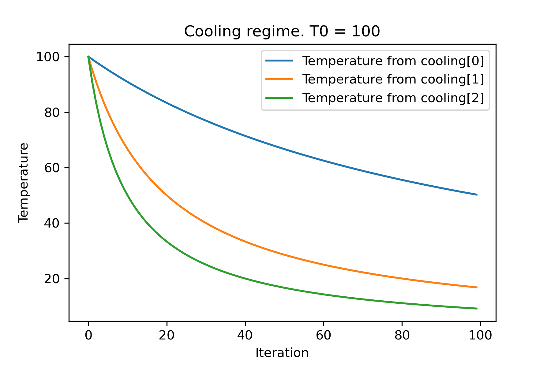
 # all supported coolling regimes

temperature = 100
cooling = [
    Cooling . linear ( mu = 1 ),
    Cooling . reverse ( beta = 0.0007 ),
    Cooling . exponential ( alpha = 0.85 ),
    Cooling . linear_reverse (),
    Cooling . logarithmic ( c = 100 , d = 1 )
    ]
SimulatedAnnealing . plot_temperature ( cooling , temperature , iterations = 100 , save_as = 'diff_temp.png' )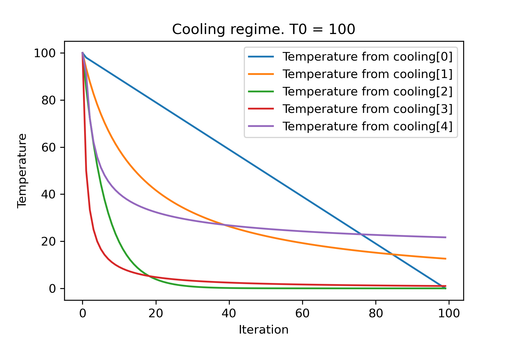
 # and we can set own temperature and cooling for each dimention!

temperature = [ 100 , 125 , 150 ]
cooling = [
    Cooling . exponential ( alpha = 0.85 ),
    Cooling . exponential ( alpha = 0.9 ),
    Cooling . exponential ( alpha = 0.95 ),
    ]
SimulatedAnnealing . plot_temperature ( cooling , temperature , iterations = 100 , save_as = 'diff_temp_and_cool.png' )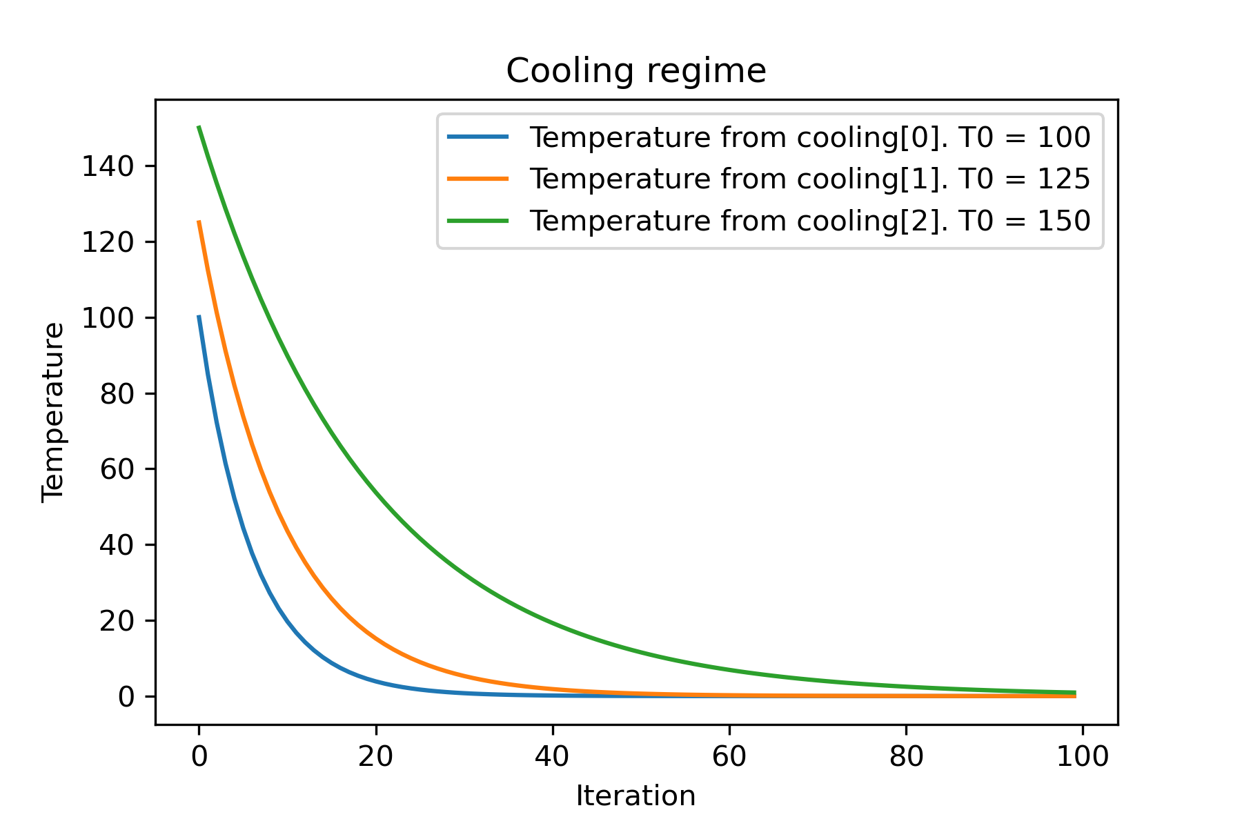
なぜそんなに多くの冷却体制があるのですか?特定のタスクでは、それらの1つがとても良い場合があります!このスクリプトでは、ラストリング機能の異なる冷却をテストできます。
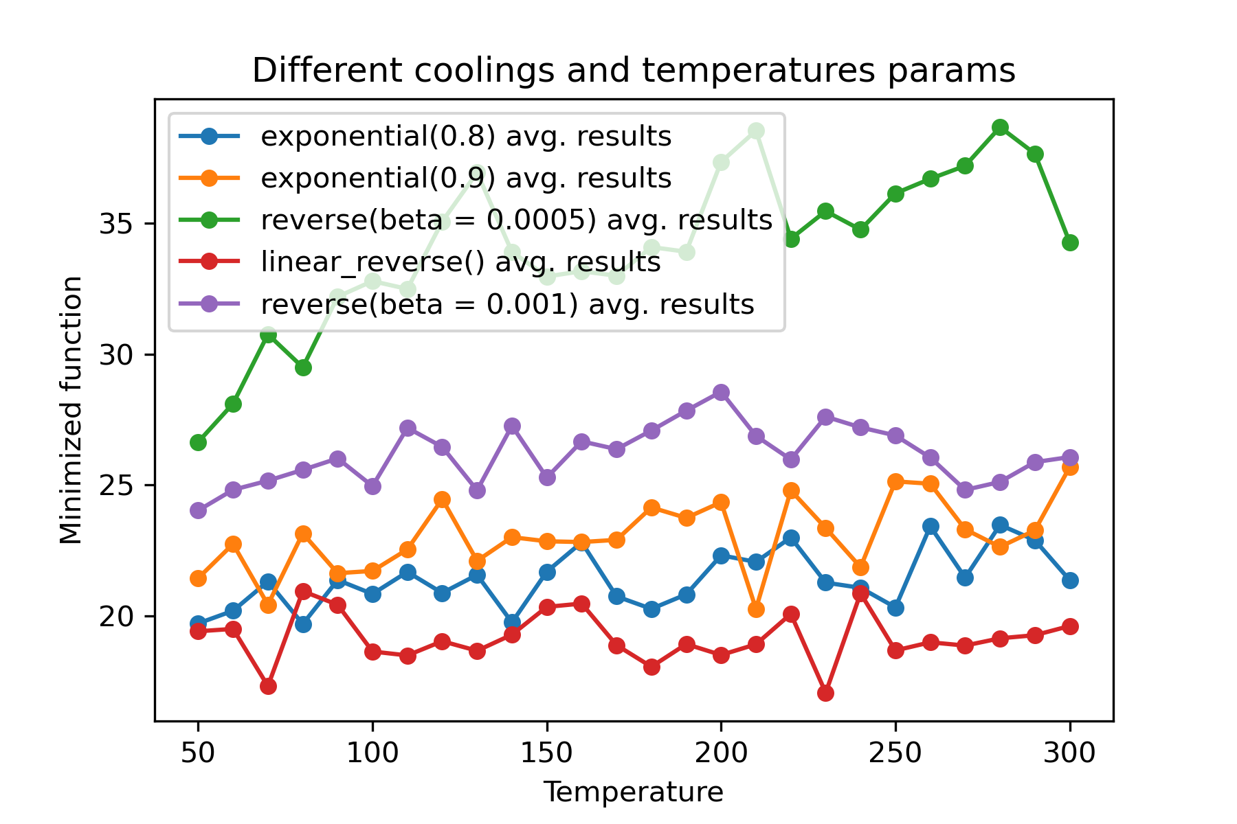
さまざまな冷却を使用し、各寸法の温度を開始することは驚くべき機能です。
 import math
import numpy as np

from SimplestSimulatedAnnleaning import SimulatedAnnealing , Cooling , simple_continual_mutation


def Rastrigin ( arr ):
    return 10 * arr . size + np . sum ( arr ** 2 ) - 10 * np . sum ( np . cos ( 2 * math . pi * arr ))

dim = 5


model = SimulatedAnnealing ( Rastrigin , dim )

best_solution , best_val = model . run (
    start_solution = np . random . uniform ( - 5 , 5 , dim ),
    mutation = simple_continual_mutation ( std = 1 ),
    cooling = [ # different cooling for each dimention
        Cooling . exponential ( 0.8 ),
        Cooling . exponential ( 0.9 ),
        Cooling . reverse ( beta = 0.0005 ),
        Cooling . linear_reverse (),
        Cooling . reverse ( beta = 0.001 )
        ],
    start_temperature = 100 ,
    max_function_evals = 1000 ,
    max_iterations_without_progress = 250 ,
    step_for_reinit_temperature = 90 ,
    reinit_from_best = False
    )

print ( best_val )

model . plot_report ( save_as = 'different_coolings.png' )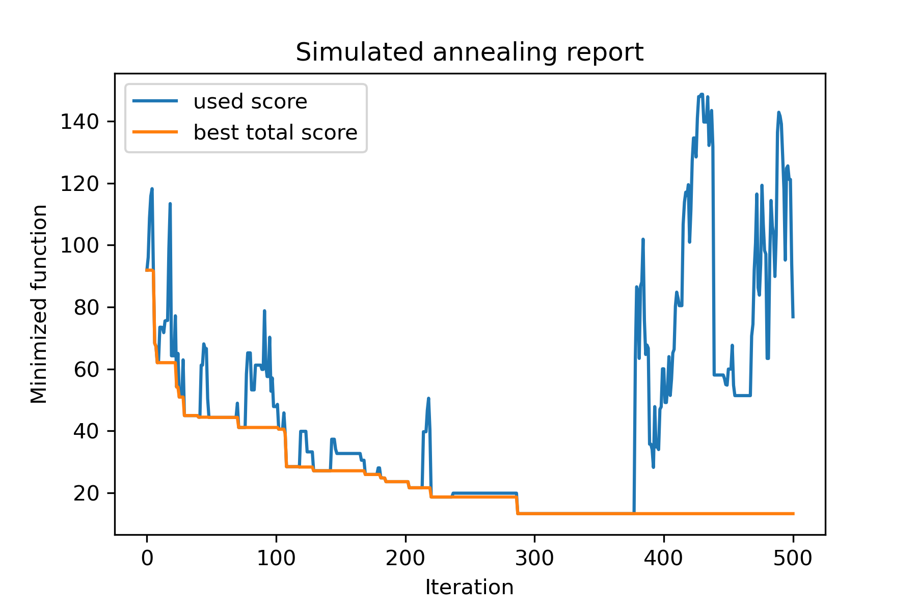
複数の冷却を使用する主な理由は、各次元の指定挙動です。たとえば、空間の最初の次元は2番目の寸法よりもはるかに広くなる可能性があるため、最初の次元でより広い検索を使用することをお勧めします。 Uは、異なるstart temperaturesを使用して異なるcoolingsを使用して、特別なmut関数を使用して生成できます。
複数の冷却を使用するもう1つの理由は、選択の方法です。複数の冷却の場合、良いソリューションと悪いソリューションの選択が各次元で適用されます。そのため、より良い解決策を見つける可能性が高くなります。
突然変異関数は最も重要なパラメーターです。現在のオブジェクトと温度に関する情報を使用して、新しいオブジェクトを作成する動作を決定します。 mut関数を作成するときは、これらの原則を数えることをお勧めします。
mutの構造を思い出しましょう:
 def mut ( x_as_array , temperature_as_array_or_one_number ):
    # some code
return new_x_as_arrayここでx_as_array現在のソリューションであり、 new_x_as_array変異したソリューションです(覚えているように、ランダムで同じ薄暗い)。また、 temperature_as_array_or_one_number 、非培養ソリューションのみであることを覚えておく必要があります。それ以外の場合は、(いくつかの冷却またはその両方のいくつかの開始温度を使用する場合)それはnumpyアレイです。例を参照してください
この例では、 nオブジェクトを使用して設定からkオブジェクトを選択する方法を示します。
 import numpy as np
from SimplestSimulatedAnnleaning import SimulatedAnnealing , Cooling

SEED = 3

np . random . seed ( SEED )

Set = np . random . uniform ( low = - 15 , high = 5 , size = 100 ) # all set

dim = 10 # how many objects should we choose

indexes = np . arange ( Set . size )
# minimized function -- subset with best |median|
def min_func ( arr ):
    return abs ( np . median ( Set [ indexes [ arr . astype ( bool )]]))

# zero vectors with 'dim' ones at random positions
start_solution = np . zeros ( Set . size )
start_solution [ np . random . choice ( indexes , dim , replace = False )] = 1

# mutation function
# temperature is the number cuz we will use only 1 cooling, but it's not necessary to use it)
def mut ( x_as_array , temperature_as_array_or_one_number ):
    mask_one = x_as_array == 1
    mask_zero = np . logical_not ( mask_one )

    new_x_as_array = x_as_array . copy ()
    # replace some zeros with ones
    new_x_as_array [ np . random . choice ( indexes [ mask_one ], 1 , replace = False )] = 0
    new_x_as_array [ np . random . choice ( indexes [ mask_zero ], 1 , replace = False )] = 1

    return new_x_as_array

# creating a model
model = SimulatedAnnealing ( min_func , dim )

# run search
best_solution , best_val = model . run (
    start_solution = start_solution ,
    mutation = mut ,
    cooling = Cooling . exponential ( 0.9 ),
    start_temperature = 100 ,
    max_function_evals = 1000 ,
    max_iterations_without_progress = 100 ,
    step_for_reinit_temperature = 80 ,
    seed = SEED
    )

model . plot_report ( save_as = 'best_subset.png' )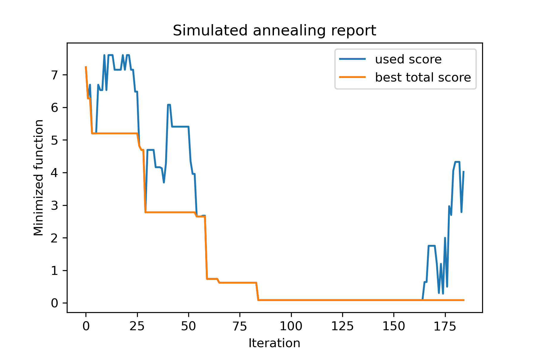
このタスクを見てみましょう。
 split set of values {v1, v2, v3, ..., vn} to sets 0, 1, 2, 3
with their sizes (volumes determined by user) to complete best sets metric
それを解決する方法の1つ:
 from collections import defaultdict
import numpy as np

from SimplestSimulatedAnnleaning import SimulatedAnnealing , Cooling

################### useful methods

def counts_to_vec ( dic_count ):
    """
    converts dictionary like {1: 3, 2: 4}
    to array [1, 1, 1, 2, 2, 2, 2]
    """
    arrs = [ np . full ( val , fill_value = key ) for key , val in dic_count . items ()]

    return np . concatenate ( tuple ( arrs ))

def vec_to_indexes_dict ( vector ):
    """
    converts vector like [1, 0, 1, 2, 2]
    to dictionary with indexes {1: [0, 2], 2: [3, 4]}
    """

    res = defaultdict ( list )

    for i , v in enumerate ( vector ):
        res [ v ]. append ( i )

    return { int ( key ): np . array ( val ) for key , val in res . items () if key != 0 }


#################### START PARAMS

SEED = 3

np . random . seed ( SEED )

Set = np . random . uniform ( low = - 15 , high = 5 , size = 100 ) # all set
Set_indexes = np . arange ( Set . size )

# how many objects should be in each set
dim_dict = {
    1 : 10 ,
    2 : 10 ,
    3 : 7 ,
    4 : 14
}


# minimized function: sum of means vy each split set
def min_func ( arr ):

    indexes_dict = vec_to_indexes_dict ( arr )

    means = [ np . mean ( Set [ val ]) for val in indexes_dict . values ()]

    return sum ( means )

# zero vector with available set labels at random positions
start_solution = np . zeros ( Set . size , dtype = np . int8 )
labels_vec = counts_to_vec ( dim_dict )
start_solution [ np . random . choice ( Set_indexes , labels_vec . size , replace = False )] = labels_vec


def choice ( count = 3 ):
    return np . random . choice ( Set_indexes , count , replace = False )

# mutation function
# temperature is the number cuz we will use only 1 cooling, but it's not necessary to use it)
def mut ( x_as_array , temperature_as_array_or_one_number ):

    new_x_as_array = x_as_array . copy ()
    # replace some values

    while True :
        inds = choice ()

        if np . unique ( new_x_as_array [ inds ]). size == 1 : # there is no sense to replace same values
            continue
        new_x_as_array [ inds ] = new_x_as_array [ np . random . permutation ( inds )]

        return new_x_as_array

# creating a model
model = SimulatedAnnealing ( min_func , Set_indexes . size )

# run search
best_solution , best_val = model . run (
    start_solution = start_solution ,
    mutation = mut ,
    cooling = Cooling . exponential ( 0.9 ),
    start_temperature = 100 ,
    max_function_evals = 1000 ,
    max_iterations_without_progress = 100 ,
    step_for_reinit_temperature = 80 ,
    seed = SEED ,
    reinit_from_best = True
    )

model . plot_report ( save_as = 'best_split.png' )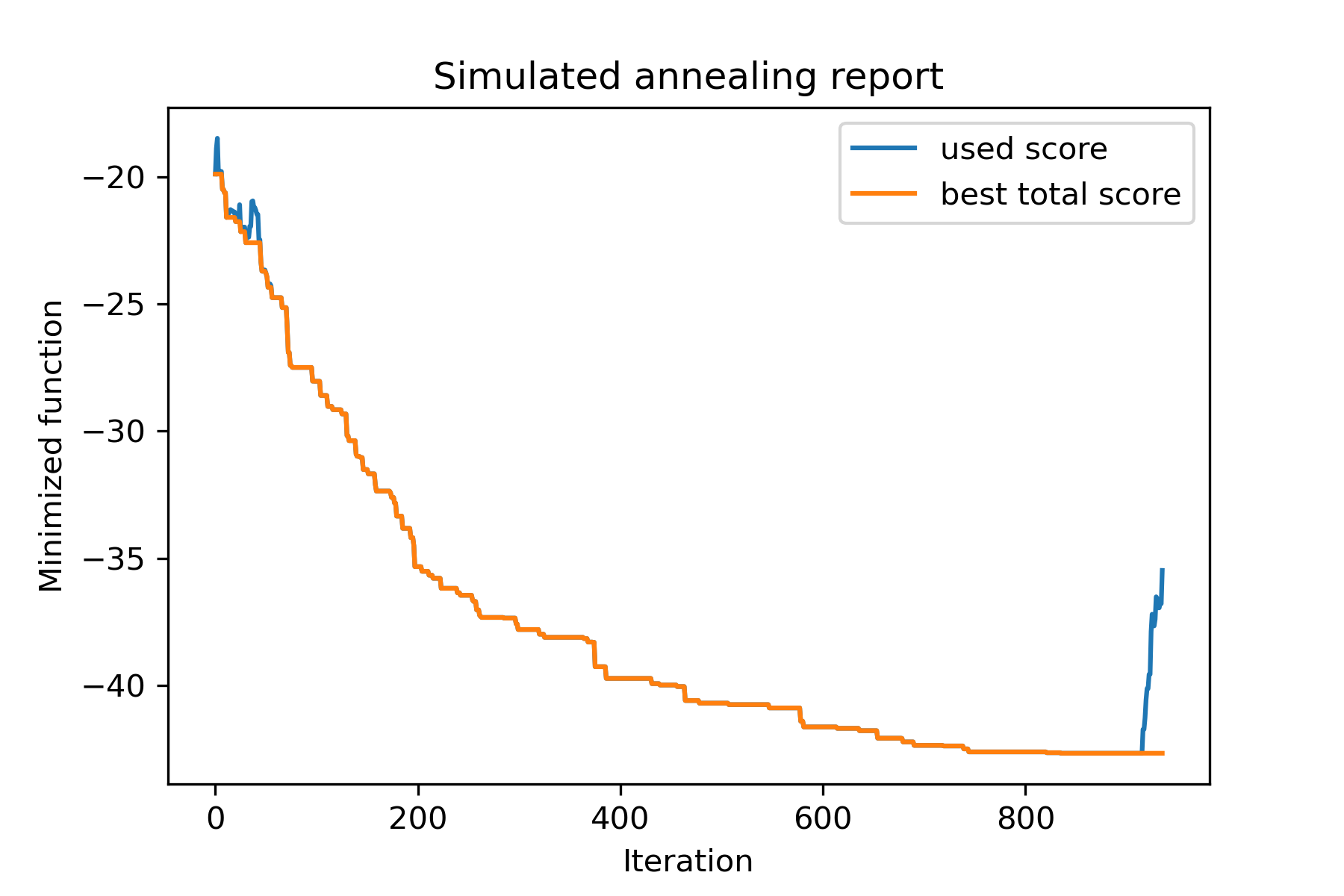
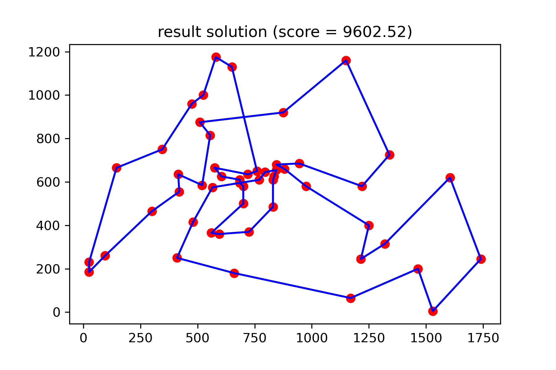
Berlin52タスクの旅行セールスマンの問題を解決してみましょう。このタスクには、ファイルから座標を持つ52の都市があります。
まず、パッケージをインポートしましょう。
 import math
import numpy as np
import pandas as pd
import matplotlib . pyplot as plt

from SimplestSimulatedAnnleaning import SimulatedAnnealing , Cooling
再現するために種子を設定します:
 SEED = 1
np . random . seed ( SEED )
座標を読み、距離マトリックスを作成します。
 # read coordinates
coords = pd . read_csv ( 'berlin52_coords.txt' , sep = ' ' , header = None , names = [ 'index' , 'x' , 'y' ])

# dim is equal to count of cities
dim = coords . shape [ 0 ]

# distance matrix
distances = np . empty (( dim , dim ))

for i in range ( dim ):
    distances [ i , i ] = 0
    for j in range ( i + 1 , dim ):
        d = math . sqrt ( np . sum (( coords . iloc [ i , 1 :] - coords . iloc [ j , 1 :]) ** 2 ))
        distances [ i , j ] = d
        distances [ j , i ] = d
ランダム開始ソリューションを作成します:
 indexes = np . arange ( dim )
# some start solution (indexes shuffle)
start_solution = np . random . choice ( indexes , dim , replace = False )
方法の長さを計算する関数を定義します。
 # minized function
def way_length ( arr ):
    s = 0
    for i in range ( 1 , dim ):
        s += distances [ arr [ i - 1 ], arr [ i ]]
    # also we should end the way in the beggining
    s += distances [ arr [ - 1 ], arr [ 1 ]]

    return s
ソリューションを視覚化しましょう:
 def plotData ( indices , title , save_as = None ):

    # create a list of the corresponding city locations:
    locs = [ coords . iloc [ i , 1 :] for i in indices ]
    locs . append ( coords . iloc [ indices [ 0 ], 1 :])

    # plot a line between each pair of consequtive cities:
    plt . plot ( * zip ( * locs ), linestyle = '-' , color = 'blue' )

    # plot the dots representing the cities:
    plt . scatter ( coords . iloc [:, 1 ], coords . iloc [:, 2 ], marker = 'o' , s = 40 , color = 'red' )
    plt . title ( title )

    if not ( save_as is None ):  plt . savefig ( save_as , dpi = 300 )

    plt . show ()


# let's plot start solution
plotData ( start_solution , f'start random solution (score = { round ( way_length ( start_solution ), 2 ) } )' , 'salesman_start.png' )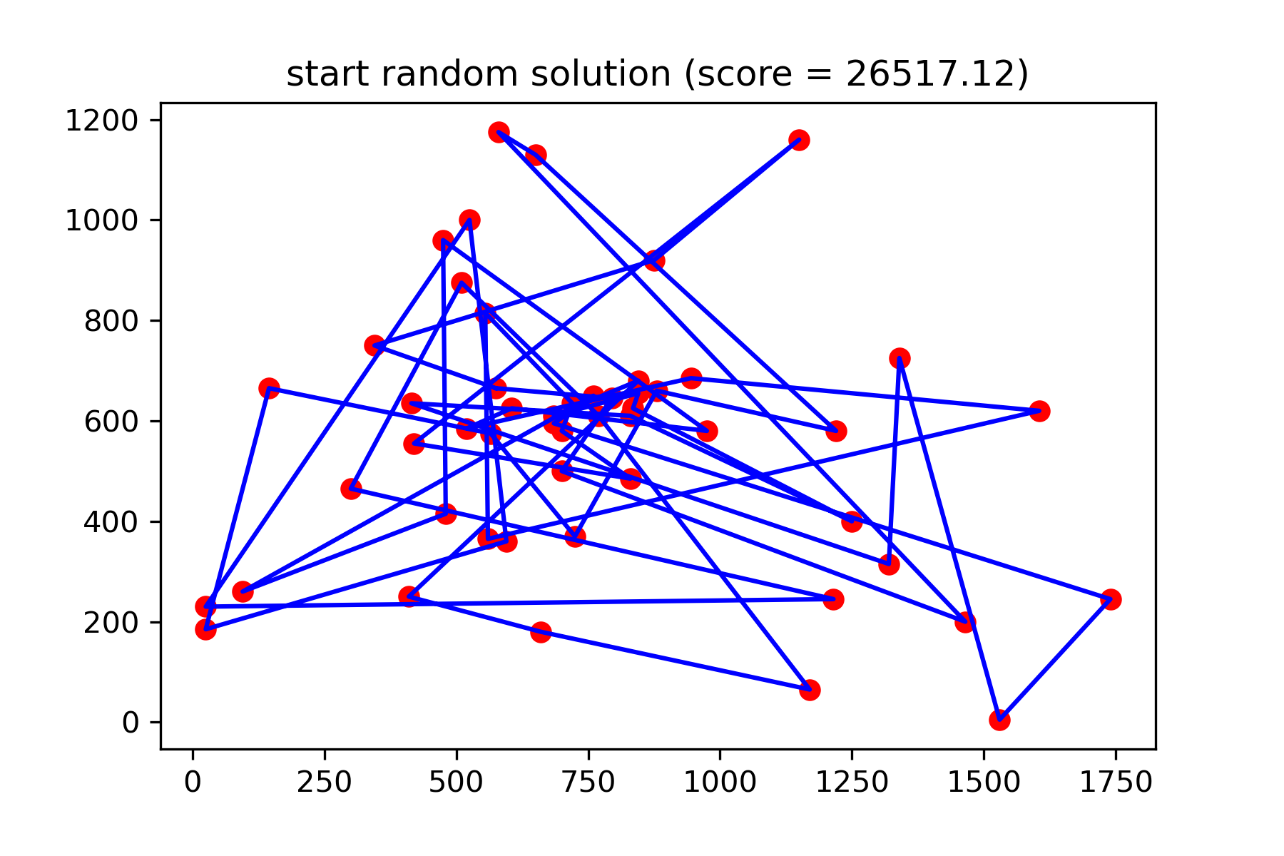
それは本当に良い解決策ではありません。このタスクのためにこの突然変異関数を作成したい:
 def mut ( x_as_array , temperature_as_array_or_one_number ):
    # random indexes
    rand_inds = np . random . choice ( indexes , 3 , replace = False )
    # shuffled indexes
    goes_to = np . random . permutation ( rand_inds )

    # just replace some positions in the array
    new_x_as_array = x_as_array . copy ()
    new_x_as_array [ rand_inds ] = new_x_as_array [ goes_to ]

    return new_x_as_array
検索を開始:
 # creating a model
model = SimulatedAnnealing ( way_length , dim )

# run search
best_solution , best_val = model . run (
    start_solution = start_solution ,
    mutation = mut ,
    cooling = Cooling . exponential ( 0.9 ),
    start_temperature = 100 ,
    max_function_evals = 15000 ,
    max_iterations_without_progress = 2000 ,
    step_for_reinit_temperature = 80 ,
    reinit_from_best = True ,
    seed = SEED
    )

model . plot_report ( save_as = 'best_salesman.png' )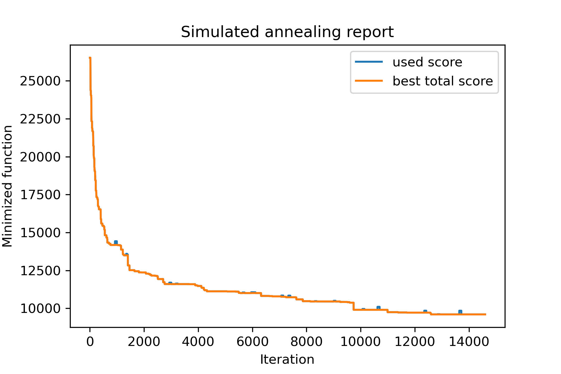
そして、私たちのもっと良い解決策を見てください:
plotData ( best_solution , f'result solution (score = { round ( best_val , 2 ) } )' , 'salesman_result.png' )