SimplestSimulatedAnnealing

أبسط الصلب محاكاة

أبسط تنفيذ (من DPEA) لطريقة الصلب المحاكاة

 pip install SimplestSimulatedAnnealing

• أبسط الصلب محاكاة
  • فكرة الطريقة
  • استخدام بسيط
  • معلمات الطريقة
  • أنظمة درجة الحرارة
    • نمط
    • الوظائف المتاحة
    • درجة حرارة المؤامرة
    • الفرق بين التبريد
    • برودة متعددة
    • إعطاء تغيير في التبريد المتعدد
  • حول طفرة
• أمثلة
  • حدد أفضل مجموعة فرعية
  • افعل أفضل انقسام
  • مشكلة البائع في السفر

فكرة الطريقة

هذه هي الخوارزمية التطورية لتقليل الوظيفة .

خطوات:

1. يجب أن نحدد الوظيفة f يجب تقليلها
2. تحديد محلول البدء x0 (يمكن أن يكون عشوائيًا)
3. تحديد وظيفة طفرة mut . يجب أن تعطي هذه الوظيفة حلًا جديدًا (يمكن أن تكون عشوائية) x1 باستخدام معلومات حول x0 ودرجة الحرارة T
4. حدد أو إنشاء نظام cooling (سلوك درجات الحرارة)
5. ضبط درجة حرارة (S) T
6. تشغيل البحث:
   • في البداية لدينا حل x0 و f(x0) أفضل درجة
   • دعنا ننشئ متحولة x1 = mut(x0) وحساب f(x1)
   • إذا كان f(x1) < f(x0) ، فقد وجدنا حل أفضل x0 = x1 . وإلا يمكننا استبدال x1 بـ x0 مع الاحتمال يساوي exp((f(x0) - f(x1)) / T)
   • انخفض T باستخدام وظيفة cooling : T = cooling(T)
   • كرر آخر 3 خطوات حتى إيقاف معيار

استخدام بسيط

حزم الاستيراد:

 import math
import numpy as np

from SimplestSimulatedAnnleaning import SimulatedAnnealing , Cooling , simple_continual_mutation

تحديد وظيفة الحد الأدنى (rastrigin):

 def Rastrigin ( arr ):
    return 10 * arr . size + np . sum ( arr ** 2 ) - 10 * np . sum ( np . cos ( 2 * math . pi * arr ))

dim = 5

سوف نستخدم أبسط طفرة غاوس:

 mut = simple_continual_mutation ( std = 0.5 )

إنشاء كائن النموذج (تعيين الوظيفة والبعد):

 model = SimulatedAnnealing ( Rastrigin , dim )

ابدأ في البحث وشاهد التقرير:

 best_solution , best_val = model . run (
    start_solution = np . random . uniform ( - 5 , 5 , dim ),
    mutation = mut ,
    cooling = Cooling . exponential ( 0.9 ), 
    start_temperature = 100 , 
    max_function_evals = 1000 , 
    max_iterations_without_progress = 100 , 
    step_for_reinit_temperature = 80
    )

model . plot_report ( save_as = 'simple_example.png' )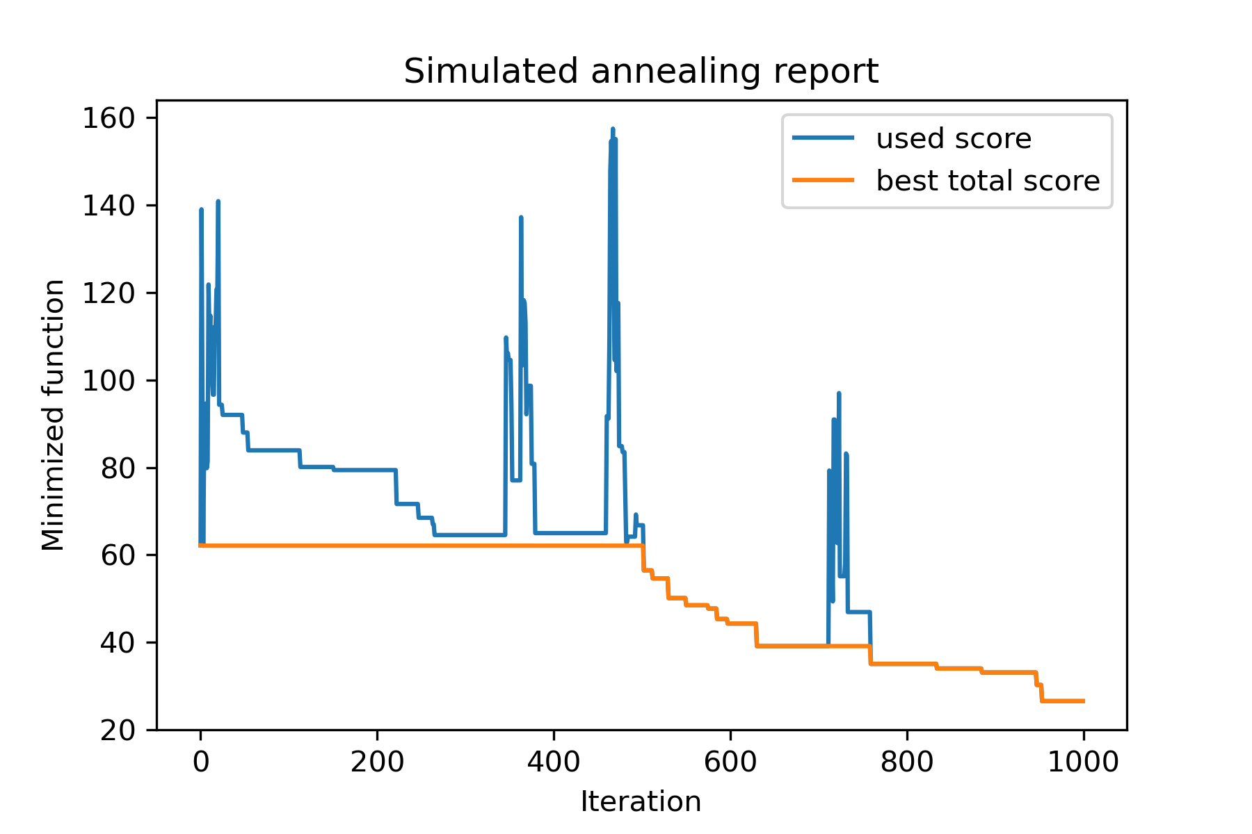

معلمات الطريقة

الطريقة الرئيسية للحزمة هي run() . دعنا نتحقق من الحجج:

 model . run ( start_solution , 
          mutation , 
          cooling , 
          start_temperature , 
          max_function_evals = 1000 , 
          max_iterations_without_progress = 250 , 
          step_for_reinit_temperature = 90 ,
          reinit_from_best = False ,
          seed = None )

أين:

• start_solution : numpy array ؛ الحل الذي يجب أن يبدأ منه.

• mutation : وظيفة (صفيف ، صفيف/رقم). وظيفة مثل

   def mut ( x_as_array , temperature_as_array_or_one_number ):
      # some code
      return new_x_as_array

  ستنشئ هذه الوظيفة حلولًا جديدة من الموجودة. انظر أيضا

• cooling : قائمة وظيفة التبريد / وظائف. وظيفة التبريد أو قائمة منها. يرى

• start_temperature : رقم أو صفيف الأرقام (قائمة/tuple). بدء درجات الحرارة. يمكن أن يكون رقم واحد أو مجموعة من الأرقام.

• max_function_evals : int ، اختياري. الحد الأقصى لعدد تقييمات الوظائف. الافتراضي هو 1000.

• max_iterations_without_progress : int ، اختياري. الحد الأقصى لعدد التكرار دون تقدم عالمي. الافتراضي هو 250.

• step_for_reinit_temperature : int ، اختياري. بعد هذا العدد من التكرار دون تقدم درجات حرارة التقدم كما هو الحال في البداية. الافتراضي هو 90.

• reinit_from_best : منطقية ، اختيارية. ابدأ خوارزمية من أفضل حل بعد درجات حرارة Reinit (أو من الحل الحالي الأخير). الافتراضي خاطئ.

• seed : int/none ، اختياري. بذرة عشوائية (إذا لزم الأمر)

أنظمة درجة الحرارة

نمط

الجزء المهم من الخوارزمية هو وظيفة التبريد . تتحكم هذه الوظيفة في قيمة درجة الحرارة التي تعتمد على رقم التكرار الحالي ودرجة الحرارة الحالية ودرجة الحرارة. يمكنك إنشاء وظيفة التبريد الخاصة بك باستخدام النمط:

 def func ( T_last , T0 , k ):
    # some code
    return T_new

هنا T_last (int/float) هي قيمة درجة الحرارة من التكرار السابق ، T0 (int/float) هي درجة حرارة البدء و k (int> 0) هي عدد التكرار. يجب استخدام بعض هذه المعلومات لإنشاء درجة حرارة جديدة T_new .

يوصى بشدة ببناء وظيفتك لإنشاء درجة حرارة إيجابية فقط.

الوظائف المتاحة

في فئة Cooling هناك العديد من وظائف التبريد:

• Cooling.linear(mu, Tmin = 0.01)
• Cooling.exponential(alpha = 0.9)
• Cooling.reverse(beta = 0.0005)
• Cooling.logarithmic(c, d = 1) - غير موصى به
• Cooling.linear_reverse()

درجة حرارة المؤامرة

يمكن أن ترى سلوك وظيفة التبريد باستخدام طريقة SimulatedAnnealing.plot_temperature . لنرى عدة أمثلة:

 from SimplestSimulatedAnnleaning import SimulatedAnnealing , Cooling


# simplest way to set cooling regime
temperature = 100
cooling = Cooling . reverse ( beta = 0.001 )
# we can temperature behaviour using this code
SimulatedAnnealing . plot_temperature ( cooling , temperature , iterations = 100 , save_as = 'reverse.png' )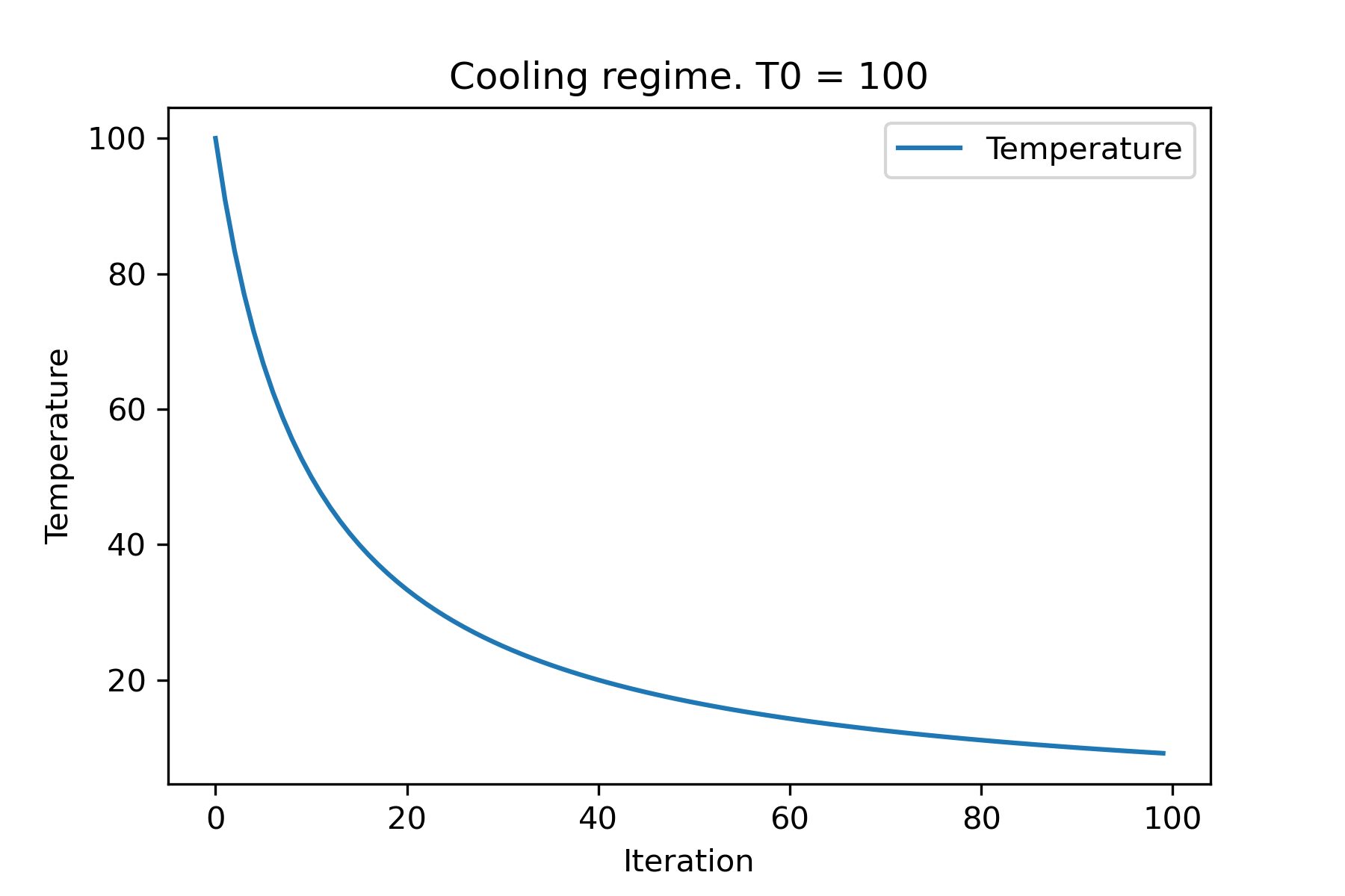

 # we can set several temparatures (for each dimention)
temperature = [ 150 , 100 , 50 ]
SimulatedAnnealing . plot_temperature ( cooling , temperature , iterations = 100 , save_as = 'reverse_diff_temp.png' )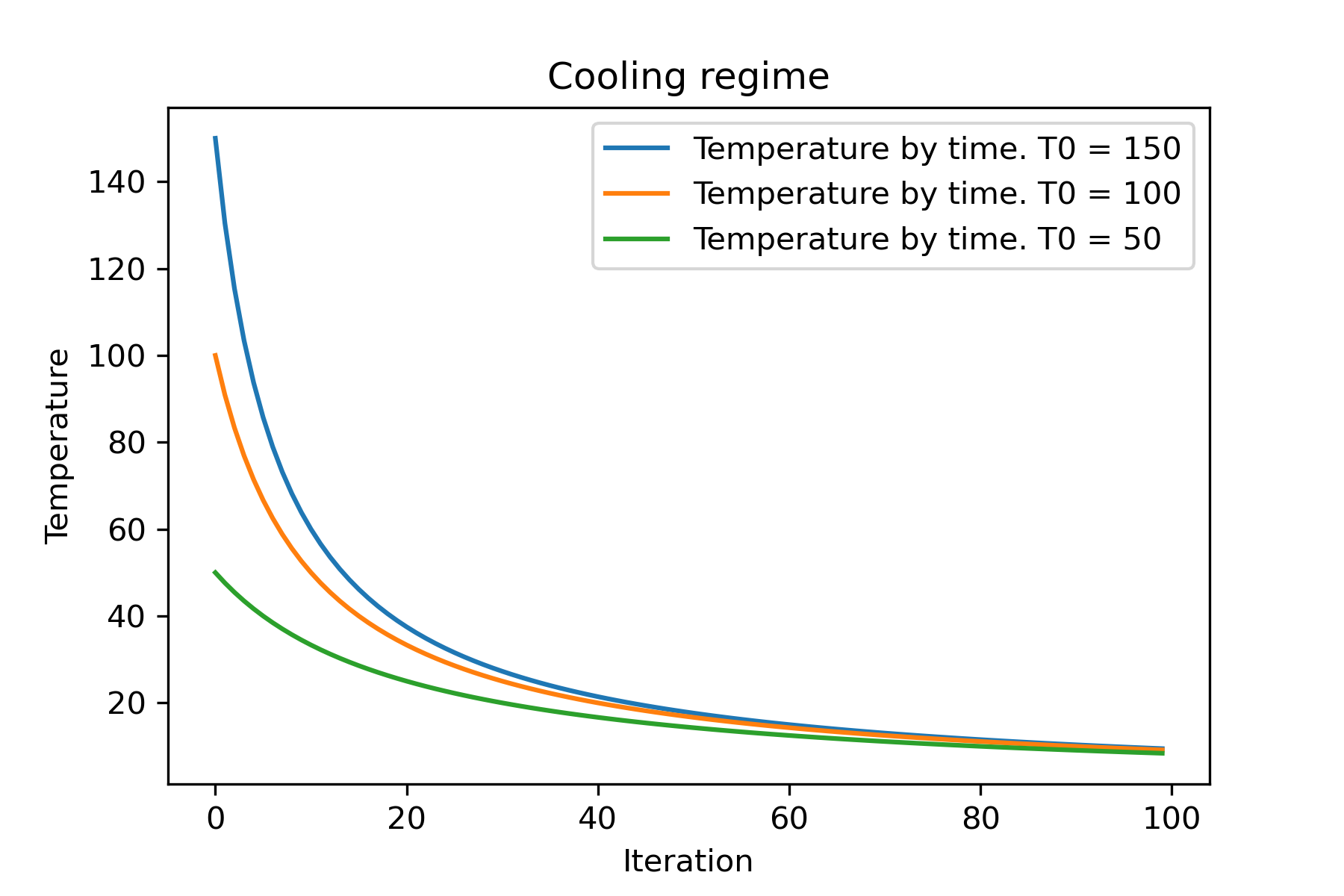

 # or several coolings (for each dimention)
temperature = 100
cooling = [
    Cooling . reverse ( beta = 0.0001 ),
    Cooling . reverse ( beta = 0.0005 ),
    Cooling . reverse ( beta = 0.001 )
    ]
SimulatedAnnealing . plot_temperature ( cooling , temperature , iterations = 100 , save_as = 'reverse_diff_beta.png' )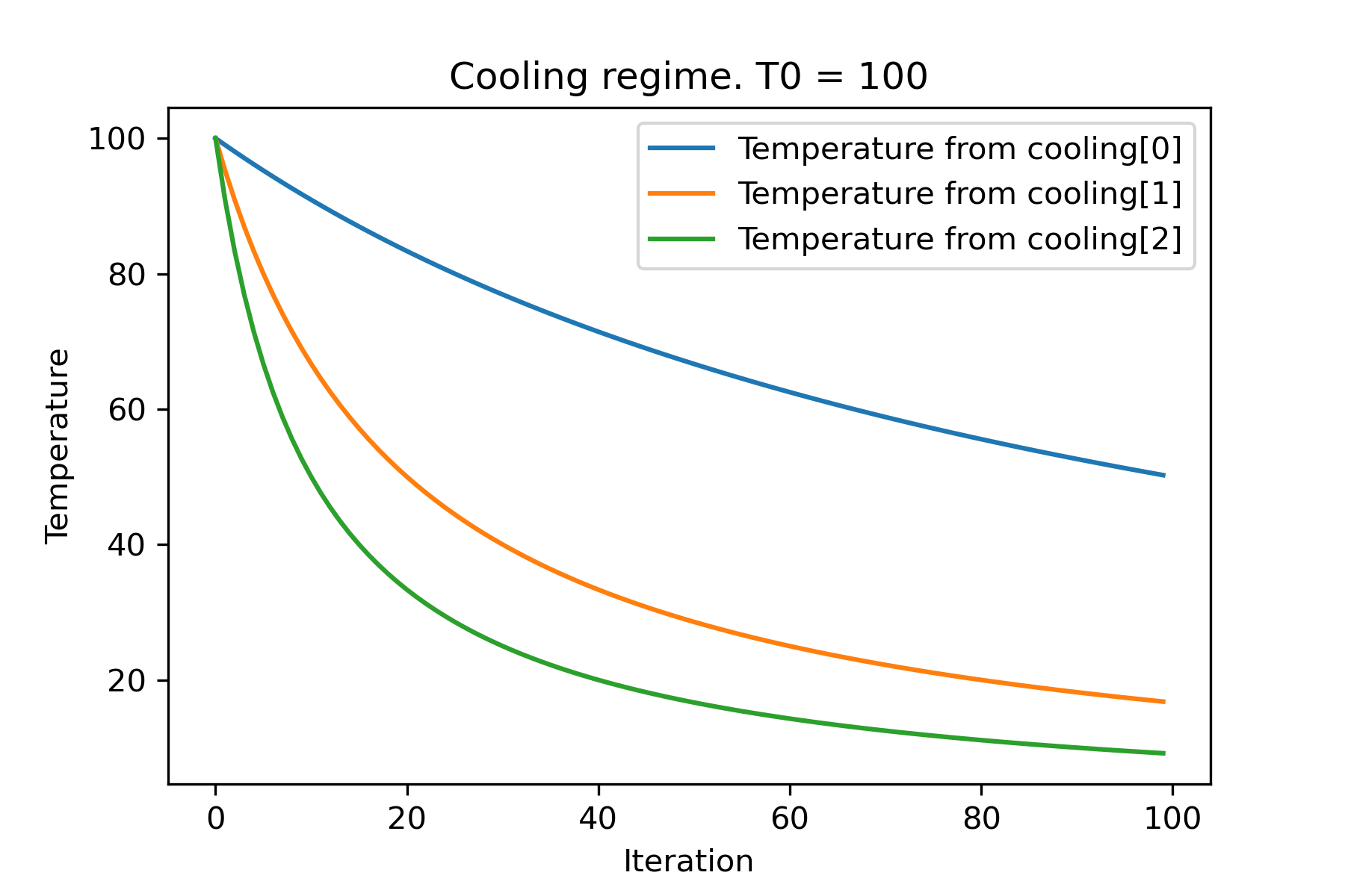

 # all supported coolling regimes

temperature = 100
cooling = [
    Cooling . linear ( mu = 1 ),
    Cooling . reverse ( beta = 0.0007 ),
    Cooling . exponential ( alpha = 0.85 ),
    Cooling . linear_reverse (),
    Cooling . logarithmic ( c = 100 , d = 1 )
    ]
SimulatedAnnealing . plot_temperature ( cooling , temperature , iterations = 100 , save_as = 'diff_temp.png' )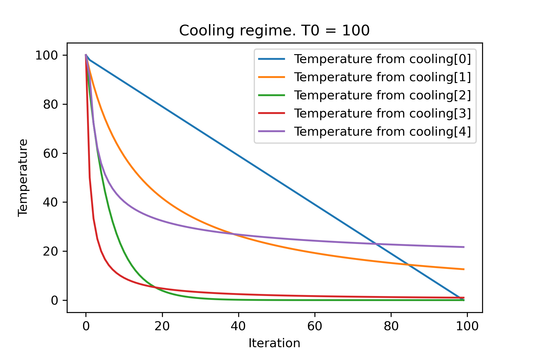

 # and we can set own temperature and cooling for each dimention!

temperature = [ 100 , 125 , 150 ]
cooling = [
    Cooling . exponential ( alpha = 0.85 ),
    Cooling . exponential ( alpha = 0.9 ),
    Cooling . exponential ( alpha = 0.95 ),
    ]
SimulatedAnnealing . plot_temperature ( cooling , temperature , iterations = 100 , save_as = 'diff_temp_and_cool.png' )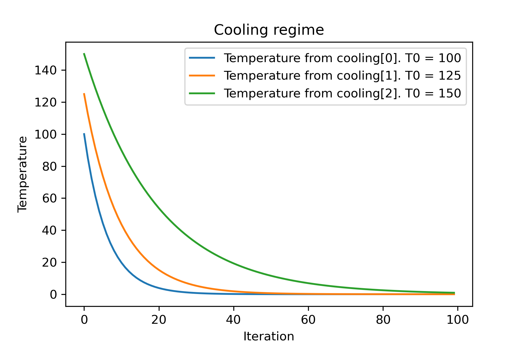

الفرق بين التبريد

لماذا هناك الكثير من أنظمة التبريد؟ لمهمة معينة يمكن أن يكون أحدهم أفضل! في هذا البرنامج النصي ، يمكننا اختبار تبريد مختلف لوظيفة Rastring:

برودة متعددة

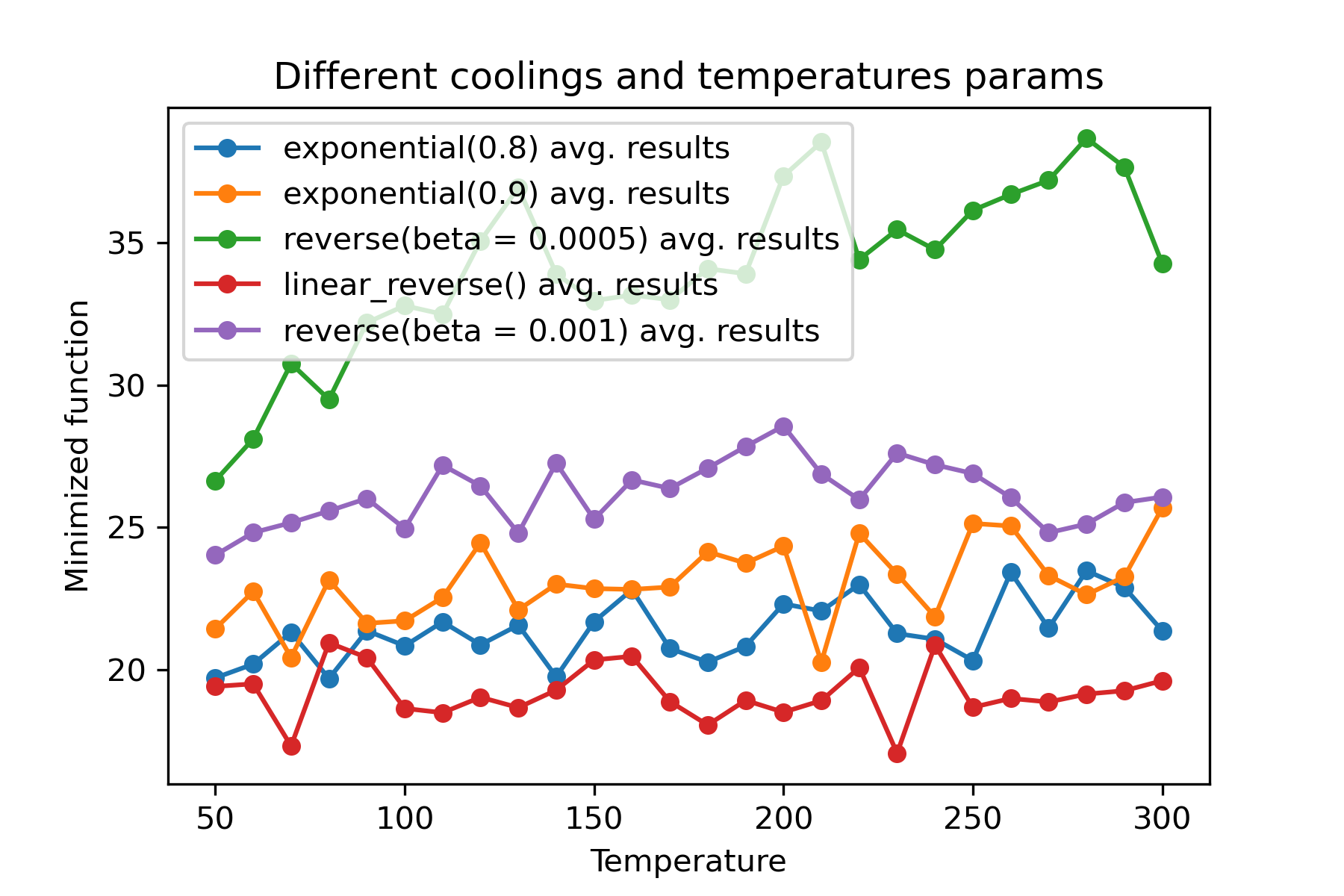
إنه لأمر مدهش استخدام تبريد مختلف وبدء درجات الحرارة لكل بعد :

 import math
import numpy as np

from SimplestSimulatedAnnleaning import SimulatedAnnealing , Cooling , simple_continual_mutation


def Rastrigin ( arr ):
    return 10 * arr . size + np . sum ( arr ** 2 ) - 10 * np . sum ( np . cos ( 2 * math . pi * arr ))

dim = 5



model = SimulatedAnnealing ( Rastrigin , dim )

best_solution , best_val = model . run (
    start_solution = np . random . uniform ( - 5 , 5 , dim ),
    mutation = simple_continual_mutation ( std = 1 ),
    cooling = [ # different cooling for each dimention
        Cooling . exponential ( 0.8 ),
        Cooling . exponential ( 0.9 ),
        Cooling . reverse ( beta = 0.0005 ),
        Cooling . linear_reverse (),
        Cooling . reverse ( beta = 0.001 )
        ], 
    start_temperature = 100 , 
    max_function_evals = 1000 , 
    max_iterations_without_progress = 250 , 
    step_for_reinit_temperature = 90 ,
    reinit_from_best = False
    )

print ( best_val )

model . plot_report ( save_as = 'different_coolings.png' )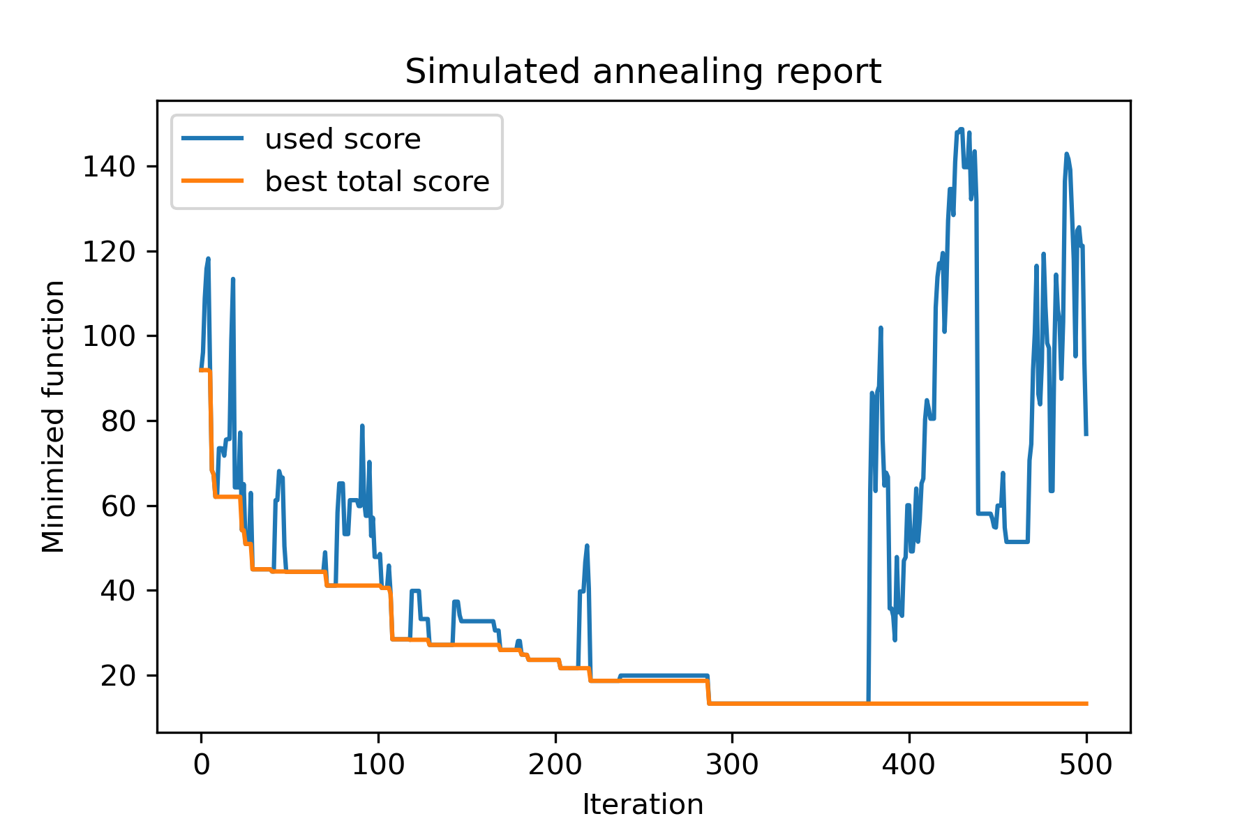

إعطاء تغيير في التبريد المتعدد

السبب الرئيسي لاستخدام التبريد المتعدد هو السلوك المحدد لكل بعد. على سبيل المثال ، يمكن أن يكون البعد الأول للمساحة أوسع بكثير من البعد الثاني ، لذلك من الأفضل استخدام البحث الأوسع عن البعد الأول ؛ يمكن أن تنتجها باستخدام وظيفة mut خاصة ، باستخدام start temperatures مختلفة واستخدام coolings مختلف.

سبب آخر لاستخدام التبريد المتعدد هو طريقة الاختيار: لاختيار التبريد المتعددة بين الحلول الجيدة والسيئة التي ينطبق عليها كل بعد . لذلك ، يزيد من فرص إيجاد حل أفضل.

حول طفرة

وظيفة الطفرة هي المعلمة الأكثر أهمية. يحدد سلوك إنشاء كائنات جديدة باستخدام معلومات حول الكائن الحالي ودرجة الحرارة. أوصي بحساب هذه المبادئ عند إنشاء وظيفة mut :

1. يجب أن يكون حل متحولة عشوائيًا ولكن "قريب" من الحل الحالي
2. يجب أن يكون محلول متحولة عادة أقرب مع انخفاض درجة الحرارة

دعونا نتذكر هيكل mut :

 def mut ( x_as_array , temperature_as_array_or_one_number ):
    # some code
    return new_x_as_array

هنا x_as_array هو الحل الحالي و new_x_as_array هو الحل المتحور (عشوائيًا ونفسه ، كما تتذكر). كما يجب أن تتذكر أن temperature_as_array_or_one_number هو الرقم فقط لمحلول غير الصدري. خلاف ذلك (عند استخدام عدة درجات حرارة بدء لعدة تبريد أو كليهما) ، فهي صفيف numpy . انظر الأمثلة

أمثلة

حدد أفضل مجموعة فرعية

في هذا المثال ، أُظهر كيفية تحديد كائنات k من SET باستخدام كائنات n التي ستقليل بعض الوظائف (في هذا المثال: القيمة المطلقة للوسيط):

 import numpy as np
from SimplestSimulatedAnnleaning import SimulatedAnnealing , Cooling

SEED = 3

np . random . seed ( SEED )

Set = np . random . uniform ( low = - 15 , high = 5 , size = 100 ) # all set

dim = 10 # how many objects should we choose

indexes = np . arange ( Set . size )
# minimized function -- subset with best |median|
def min_func ( arr ):
    return abs ( np . median ( Set [ indexes [ arr . astype ( bool )]]))

# zero vectors with 'dim' ones at random positions 
start_solution = np . zeros ( Set . size )
start_solution [ np . random . choice ( indexes , dim , replace = False )] = 1

# mutation function
# temperature is the number cuz we will use only 1 cooling, but it's not necessary to use it)
def mut ( x_as_array , temperature_as_array_or_one_number ):
    mask_one = x_as_array == 1
    mask_zero = np . logical_not ( mask_one )

    new_x_as_array = x_as_array . copy ()
    # replace some zeros with ones
    new_x_as_array [ np . random . choice ( indexes [ mask_one ], 1 , replace = False )] = 0
    new_x_as_array [ np . random . choice ( indexes [ mask_zero ], 1 , replace = False )] = 1

    return new_x_as_array

# creating a model
model = SimulatedAnnealing ( min_func , dim )

# run search
best_solution , best_val = model . run (
    start_solution = start_solution ,
    mutation = mut ,
    cooling = Cooling . exponential ( 0.9 ), 
    start_temperature = 100 , 
    max_function_evals = 1000 , 
    max_iterations_without_progress = 100 , 
    step_for_reinit_temperature = 80 ,
    seed = SEED
    )

model . plot_report ( save_as = 'best_subset.png' )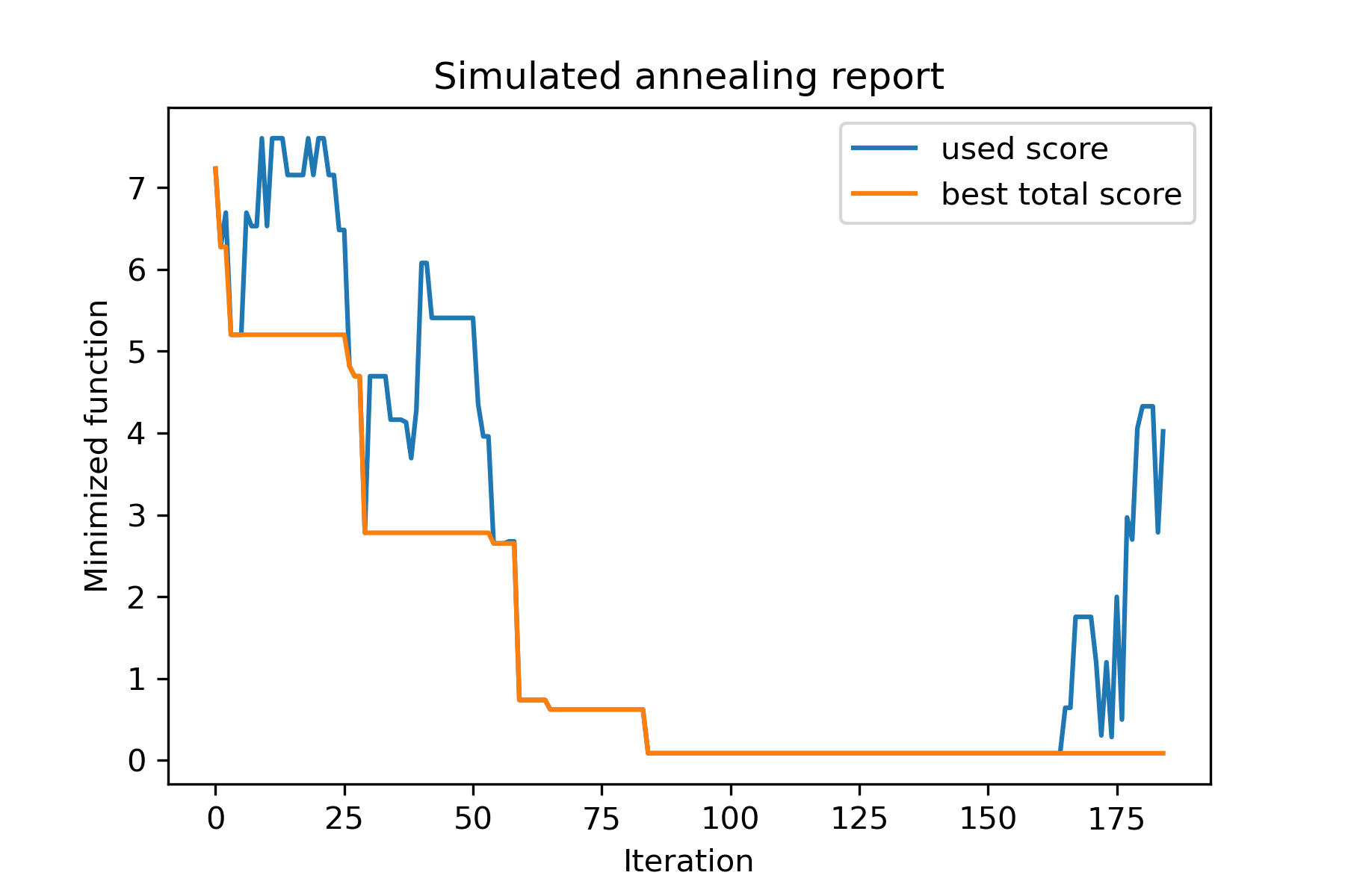

افعل أفضل انقسام

لنلقي نظرة على هذه المهمة:

 split set of values {v1, v2, v3, ..., vn} to sets 0, 1, 2, 3
with their sizes (volumes determined by user) to complete best sets metric

إحدى طرق حلها:

 from collections import defaultdict
import numpy as np

from SimplestSimulatedAnnleaning import SimulatedAnnealing , Cooling

################### useful methods

def counts_to_vec ( dic_count ):
    """
    converts dictionary like {1: 3, 2: 4}
    to array [1, 1, 1, 2, 2, 2, 2]
    """
    arrs = [ np . full ( val , fill_value = key ) for key , val in dic_count . items ()]

    return np . concatenate ( tuple ( arrs ))

def vec_to_indexes_dict ( vector ):
    """
    converts vector like [1, 0, 1, 2, 2]
    to dictionary with indexes {1: [0, 2], 2: [3, 4]}
    """

    res = defaultdict ( list )

    for i , v in enumerate ( vector ):
        res [ v ]. append ( i )
    
    return { int ( key ): np . array ( val ) for key , val in res . items () if key != 0 }


#################### START PARAMS

SEED = 3

np . random . seed ( SEED )

Set = np . random . uniform ( low = - 15 , high = 5 , size = 100 ) # all set
Set_indexes = np . arange ( Set . size )

# how many objects should be in each set
dim_dict = {
    1 : 10 ,
    2 : 10 ,
    3 : 7 ,
    4 : 14
}


# minimized function: sum of means vy each split set
def min_func ( arr ):

    indexes_dict = vec_to_indexes_dict ( arr )

    means = [ np . mean ( Set [ val ]) for val in indexes_dict . values ()]

    return sum ( means )

# zero vector with available set labels at random positions 
start_solution = np . zeros ( Set . size , dtype = np . int8 )
labels_vec = counts_to_vec ( dim_dict )
start_solution [ np . random . choice ( Set_indexes , labels_vec . size , replace = False )] = labels_vec


def choice ( count = 3 ):
    return np . random . choice ( Set_indexes , count , replace = False )

# mutation function
# temperature is the number cuz we will use only 1 cooling, but it's not necessary to use it)
def mut ( x_as_array , temperature_as_array_or_one_number ):

    new_x_as_array = x_as_array . copy ()
    # replace some values

    while True :
        inds = choice ()

        if np . unique ( new_x_as_array [ inds ]). size == 1 : # there is no sense to replace same values
            continue
        new_x_as_array [ inds ] = new_x_as_array [ np . random . permutation ( inds )]

        return new_x_as_array

# creating a model
model = SimulatedAnnealing ( min_func , Set_indexes . size )

# run search
best_solution , best_val = model . run (
    start_solution = start_solution ,
    mutation = mut ,
    cooling = Cooling . exponential ( 0.9 ), 
    start_temperature = 100 , 
    max_function_evals = 1000 , 
    max_iterations_without_progress = 100 , 
    step_for_reinit_temperature = 80 ,
    seed = SEED ,
    reinit_from_best = True
    )

model . plot_report ( save_as = 'best_split.png' )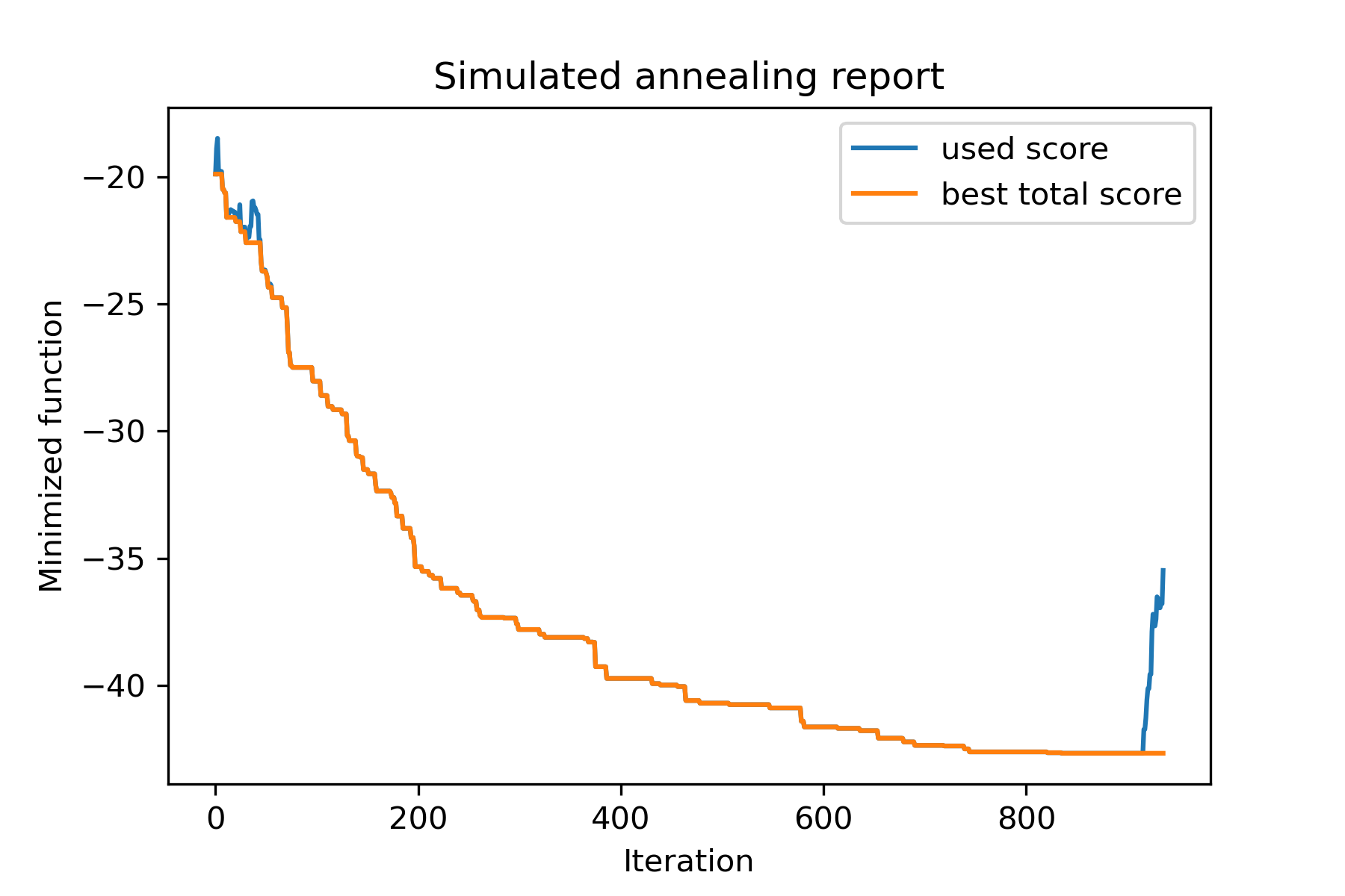

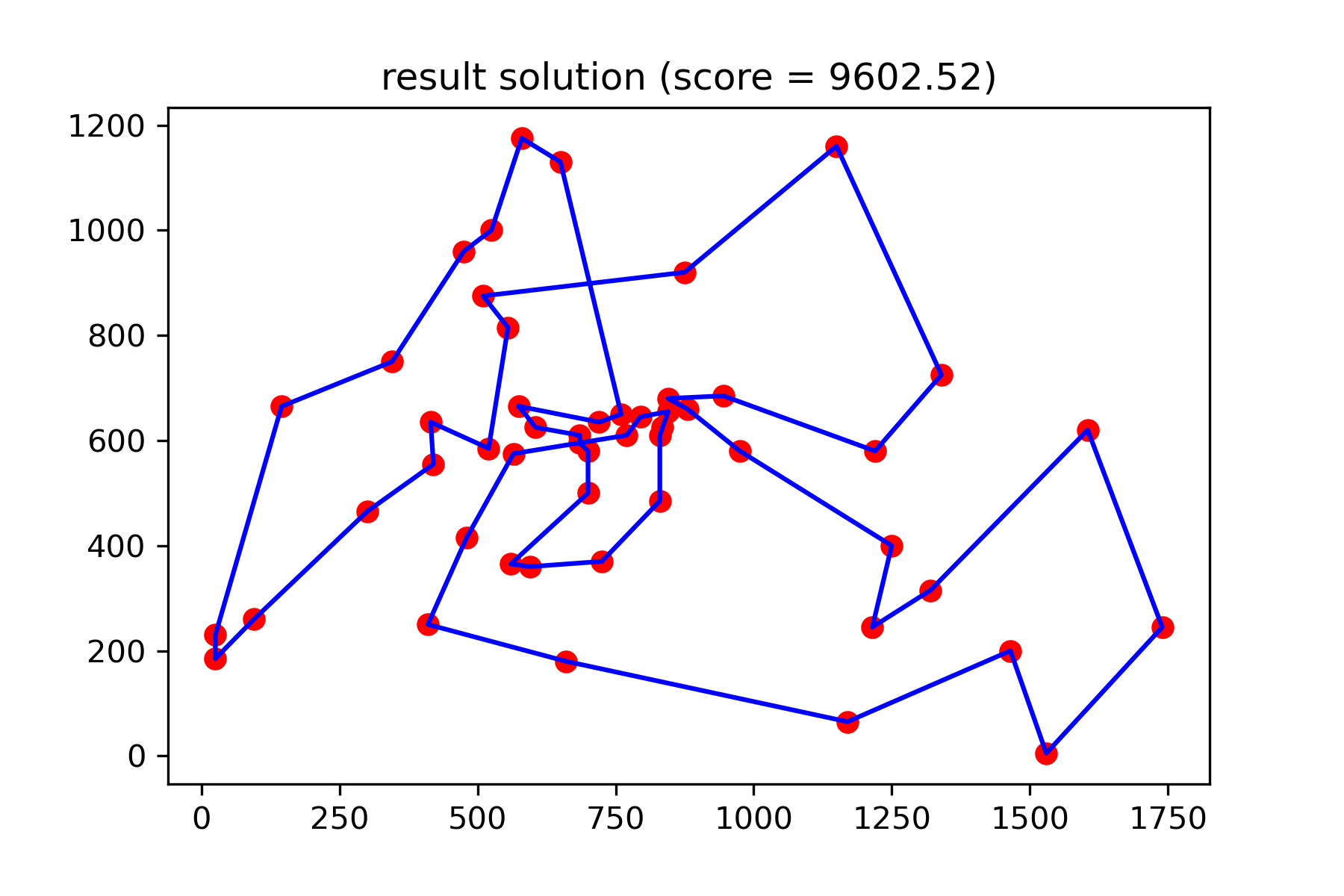
مشكلة البائع في السفر

دعنا نحاول حل مشكلة البائع المتجول لمهمة Berlin52. في هذه المهمة ، هناك 52 مدينة مع إحداثيات من الملف.

أولاً ، دعونا نستورد الحزم:

 import math
import numpy as np
import pandas as pd
import matplotlib . pyplot as plt

from SimplestSimulatedAnnleaning import SimulatedAnnealing , Cooling

تعيين بذرة للتكاثر:

 SEED = 1
np . random . seed ( SEED )

اقرأ الإحداثيات وإنشاء مصفوفة عن بعد:

 # read coordinates
coords = pd . read_csv ( 'berlin52_coords.txt' , sep = ' ' , header = None , names = [ 'index' , 'x' , 'y' ])

# dim is equal to count of cities
dim = coords . shape [ 0 ]

# distance matrix
distances = np . empty (( dim , dim ))

for i in range ( dim ):
    distances [ i , i ] = 0
    for j in range ( i + 1 , dim ):
        d = math . sqrt ( np . sum (( coords . iloc [ i , 1 :] - coords . iloc [ j , 1 :]) ** 2 ))
        distances [ i , j ] = d
        distances [ j , i ] = d

إنشاء حل عشوائي البداية:

 indexes = np . arange ( dim )
# some start solution (indexes shuffle)
start_solution = np . random . choice ( indexes , dim , replace = False )

تحديد وظيفة تحسب طول الطريق:

 # minized function
def way_length ( arr ):
    s = 0
    for i in range ( 1 , dim ):
        s += distances [ arr [ i - 1 ], arr [ i ]]
    # also we should end the way in the beggining
    s += distances [ arr [ - 1 ], arr [ 1 ]]

    return s

دعنا نتصور حل البدء:

 def plotData ( indices , title , save_as = None ):
    
    # create a list of the corresponding city locations:
    locs = [ coords . iloc [ i , 1 :] for i in indices ]
    locs . append ( coords . iloc [ indices [ 0 ], 1 :])

    # plot a line between each pair of consequtive cities:
    plt . plot ( * zip ( * locs ), linestyle = '-' , color = 'blue' )
    
    # plot the dots representing the cities:
    plt . scatter ( coords . iloc [:, 1 ], coords . iloc [:, 2 ], marker = 'o' , s = 40 , color = 'red' )    
    plt . title ( title )
    
    if not ( save_as is None ):  plt . savefig ( save_as , dpi = 300 )

    plt . show ()


# let's plot start solution
plotData ( start_solution , f'start random solution (score = { round ( way_length ( start_solution ), 2 ) } )' , 'salesman_start.png' )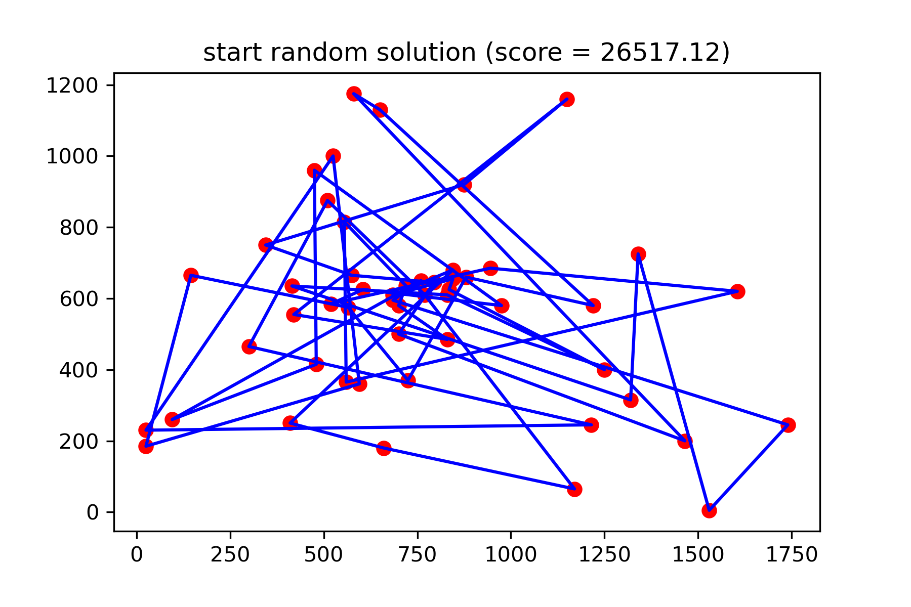

إنه حقًا ليس حلًا جيدًا. أريد إنشاء وظيفة طفرة لهذه المهمة:

 def mut ( x_as_array , temperature_as_array_or_one_number ):
    # random indexes
    rand_inds = np . random . choice ( indexes , 3 , replace = False )
    # shuffled indexes
    goes_to = np . random . permutation ( rand_inds )

    # just replace some positions in the array
    new_x_as_array = x_as_array . copy ()
    new_x_as_array [ rand_inds ] = new_x_as_array [ goes_to ]

    return new_x_as_array

ابدأ في البحث:

 # creating a model
model = SimulatedAnnealing ( way_length , dim )

# run search
best_solution , best_val = model . run (
    start_solution = start_solution ,
    mutation = mut ,
    cooling = Cooling . exponential ( 0.9 ), 
    start_temperature = 100 , 
    max_function_evals = 15000 , 
    max_iterations_without_progress = 2000 , 
    step_for_reinit_temperature = 80 ,
    reinit_from_best = True ,
    seed = SEED
    )

model . plot_report ( save_as = 'best_salesman.png' )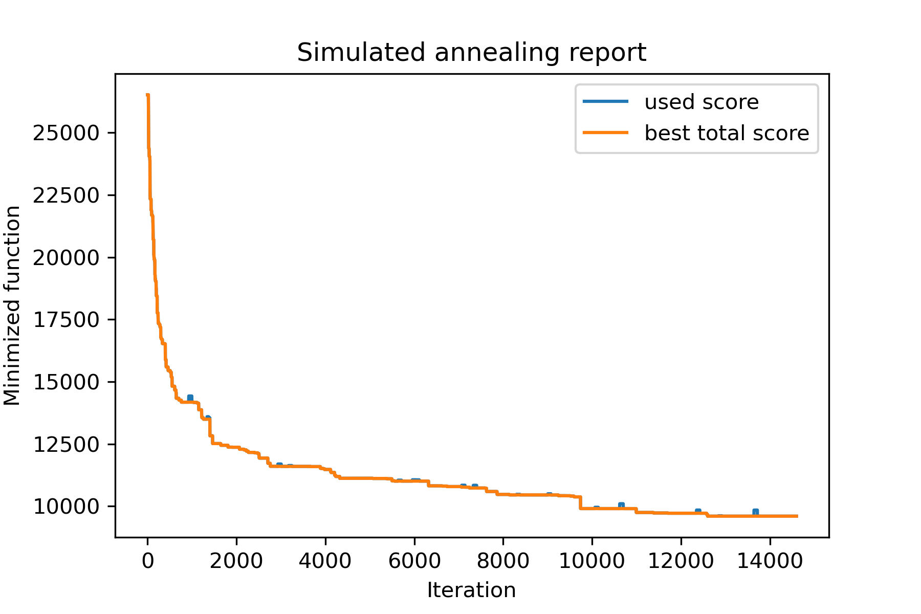

ونرى حلنا أفضل بكثير:

 plotData ( best_solution , f'result solution (score = { round ( best_val , 2 ) } )' , 'salesman_result.png' )