xai

Xai-機械学習用の説明可能性ツールボックス

Xaiは、そのコアでAIの説明可能性で設計された機械学習ライブラリです。 Xaiには、データとモデルの分析と評価を可能にするさまざまなツールが含まれています。 XAIライブラリは、倫理的AI＆ML研究所によって維持されており、責任ある機械学習の8つの原則に基づいて開発されました。

https://ethicalml.github.io/xai/index.htmlでドキュメントを見つけることができます。また、アイデアが最初に考えられたTensorflow Londonで講演をチェックすることもできます。この講演には、このライブラリの定義と原則に関する洞察も含まれています。

Xaiを使用して望ましくないバイアスを緩和する方法を示すYouTubeビデオ

Pydata London 2019 Conferenceで発表されたこの講演のビデオでは、機械学習の説明可能性の動機と、説明可能性を導入し、Xaiライブラリを使用して望ましくないバイアスを緩和する手法について概要を説明します。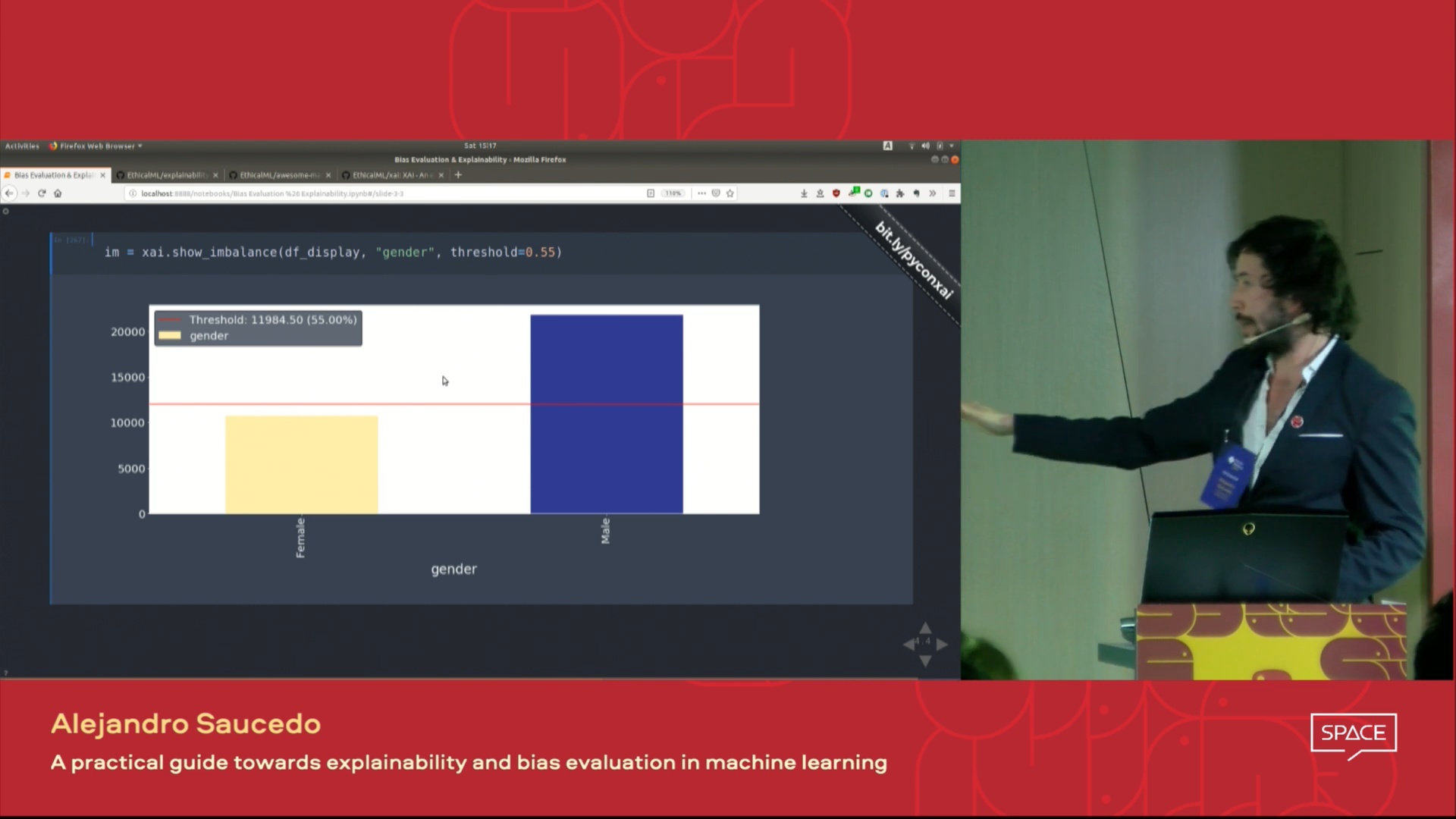
より素晴らしい機械学習の説明可能性ツールについて学びたいですか？説明可能性、プライバシー、オーケストレーションなどのためのツールの広範なリストを含むコミュニティが構築した「Awesome Machine Learning Production＆Operations」リストをご覧ください。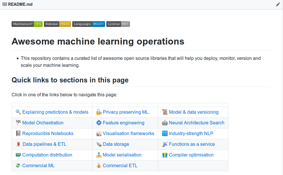

0.1.0

Actionの完全に機能的なデモを表示したい場合は、このリポジトリのクローンを作成し、ExamplesフォルダーでJupyterノートブックの例を実行します。

説明可能なAIとはどういう意味ですか？

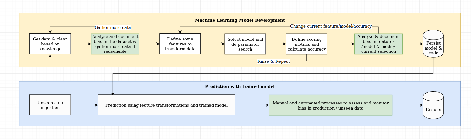
説明可能性の課題は、データサイエンスのベストプラクティスとドメイン固有の知識の組み合わせを必要とする単なるアルゴリズムの課題以上のものと考えています。 Xaiライブラリは、機械学習エンジニアと関連するドメインの専門家がエンドツーエンドのソリューションを分析し、必要な目的と比較して最適下のパフォーマンスをもたらす可能性のある矛盾を特定できるように設計されています。さらに広く言えば、Xaiライブラリは、1）データ分析、2）モデル評価、および3）生産モニタリングを含む、説明可能な機械学習の3段階を使用して設計されています。

この図で上記のこれらの3つのステップの視覚的概要を説明します。

Xai QuickStart

インストール

XaiパッケージはPypiにあります。インストールするには、実行できます。

 pip install xai

または、リポジトリをクローニングして実行して、ソースからインストールできます。

 python setup.py install 

使用法

例フォルダーに使用する例を見つけることができます。

1）データ分析

Xaiを使用すると、データの不均衡を特定できます。このために、Xaiライブラリから国勢調査データセットをロードします。

 import xai . data
df = xai . data . load_census ()
df . head ()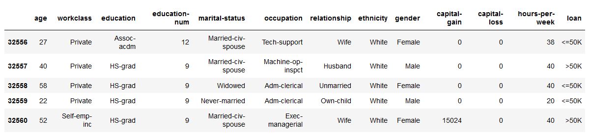

1つの列のすべてのカテゴリのクラスの不均衡を表示します

 ims = xai . imbalance_plot ( df , "gender" )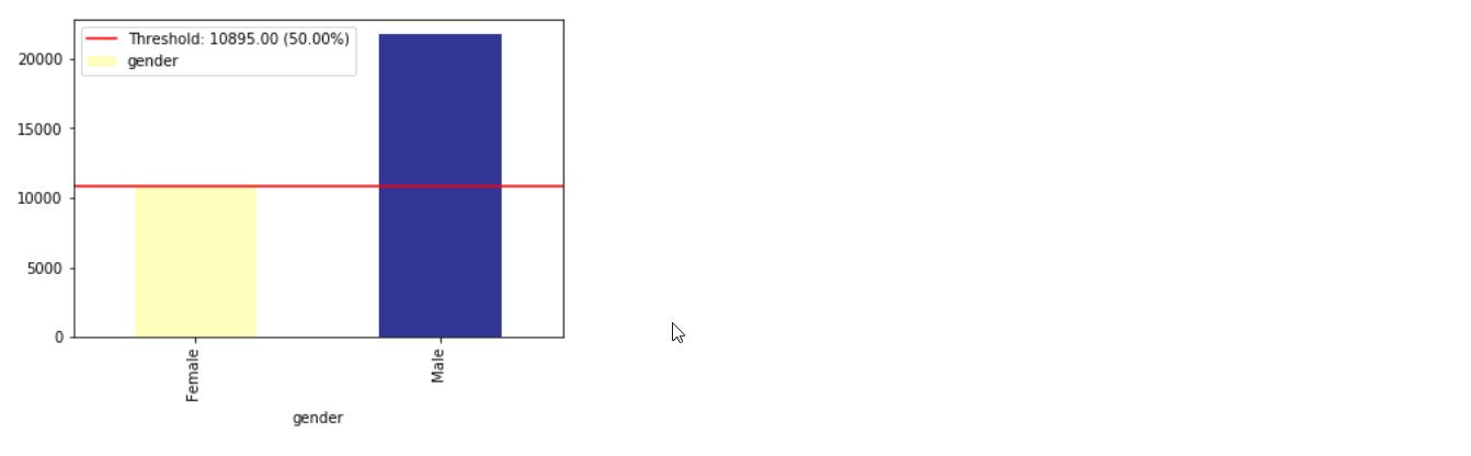

複数の列にわたってすべてのカテゴリの不均衡を表示します

 im = xai . imbalance_plot ( df , "gender" , "loan" )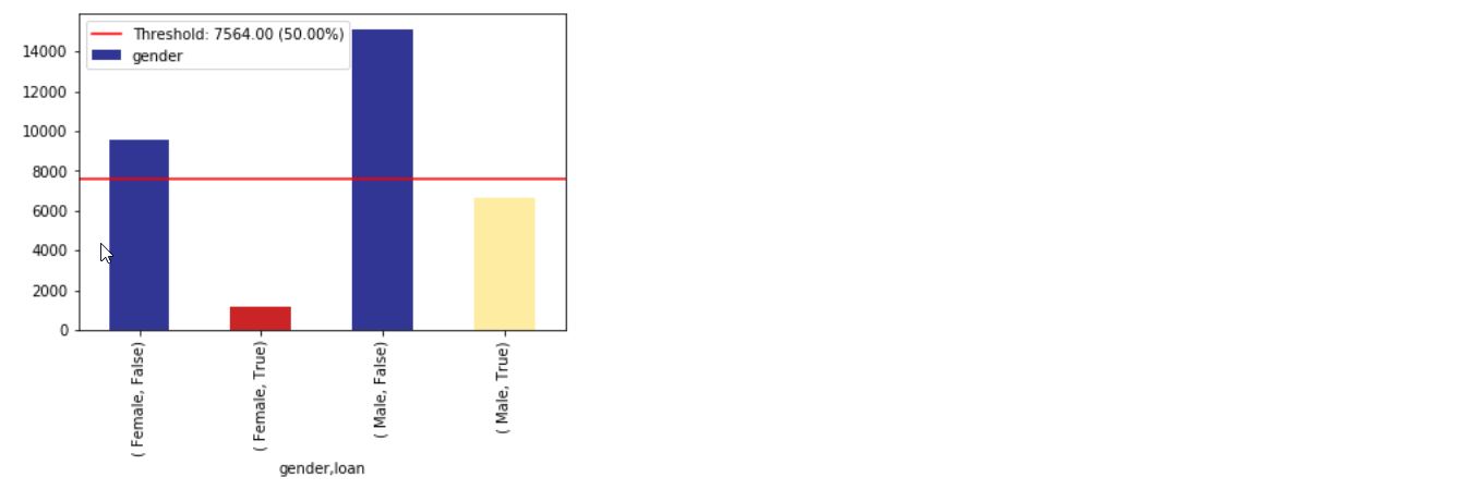

アップサンプリングおよび/またはダウンサンプリングを使用したバランスクラス

 bal_df = xai . balance ( df , "gender" , "loan" , upsample = 0.8 )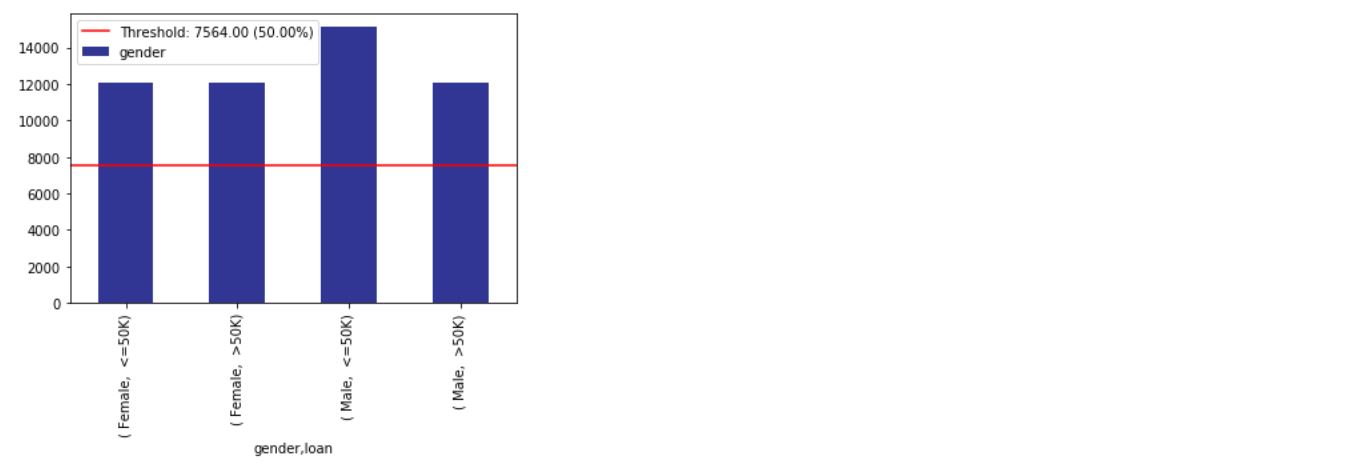

グループでカスタムオペレーションを実行します

 groups = xai . group_by_columns ( df , [ "gender" , "loan" ])
for group , group_df in groups :    
    print ( group ) 
    print ( group_df [ "loan" ]. head (), " n " )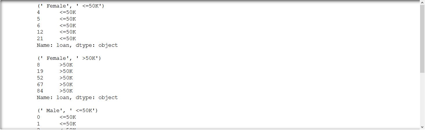

相関をマトリックスとして視覚化します

 _ = xai . correlations ( df , include_categorical = True , plot_type = "matrix" )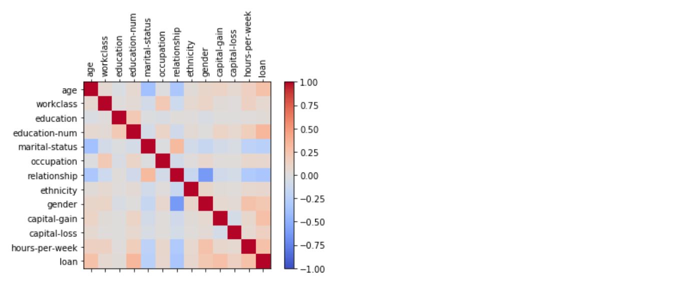

相関を階層ゼンドグラムとして視覚化します

 _ = xai . correlations ( df , include_categorical = True )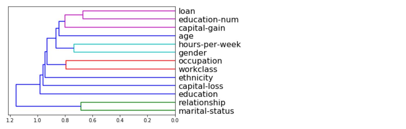

バランスの取れた検証とトレーニング分割データセットを作成します

 # Balanced train-test split with minimum 300 examples of 
#     the cross of the target y and the column gender
x_train , y_train , x_test , y_test , train_idx , test_idx = 
    xai . balanced_train_test_split (
            x , y , "gender" , 
            min_per_group = 300 ,
            max_per_group = 300 ,
            categorical_cols = categorical_cols )

x_train_display = bal_df [ train_idx ]
x_test_display = bal_df [ test_idx ]

print ( "Total number of examples: " , x_test . shape [ 0 ])

df_test = x_test_display . copy ()
df_test [ "loan" ] = y_test

_ = xai . imbalance_plot ( df_test , "gender" , "loan" , categorical_cols = categorical_cols )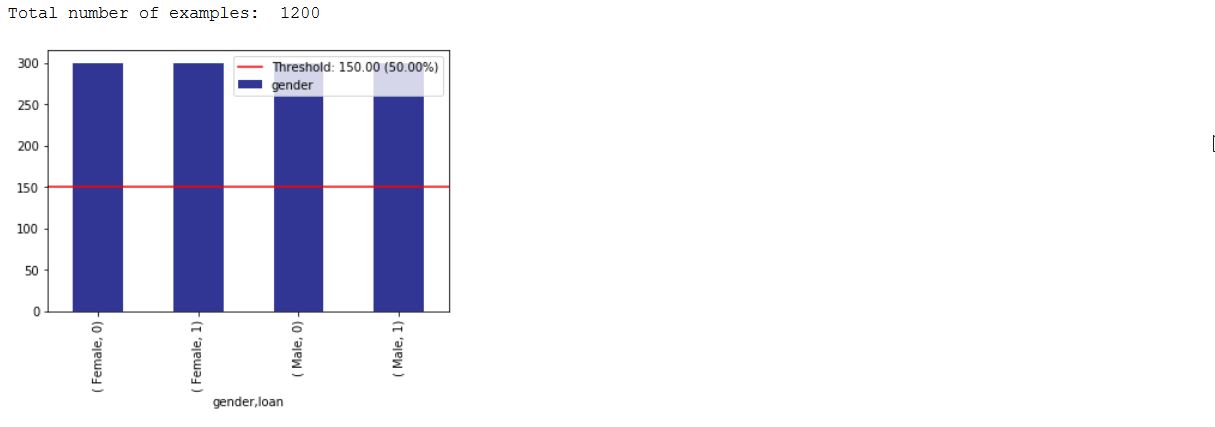

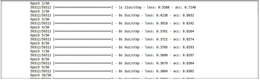
2）モデル評価

また、推論の結果と入力機能との相互作用を分析することもできます。このために、単一層の深い学習モデルをトレーニングします。

 model = build_model(proc_df.drop("loan", axis=1))

model.fit(f_in(x_train), y_train, epochs=50, batch_size=512)

probabilities = model.predict(f_in(x_test))
predictions = list((probabilities >= 0.5).astype(int).T[0])

順列機能の重要性を視覚化します

 def get_avg ( x , y ):
    return model . evaluate ( f_in ( x ), y , verbose = 0 )[ 1 ]

imp = xai . feature_importance ( x_test , y_test , get_avg )

imp . head ()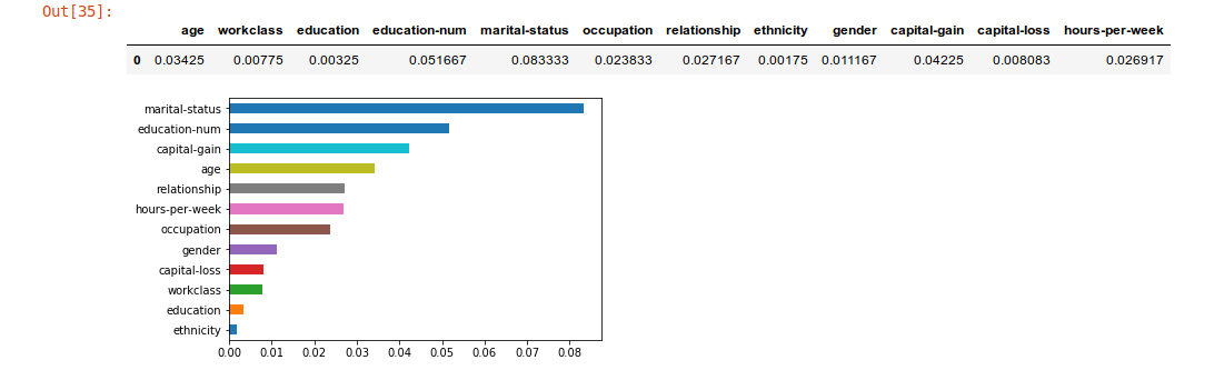

すべてのテストデータに対するメトリックの不均衡を特定します

 _ = xai . metrics_plot (
        y_test , 
        probabilities )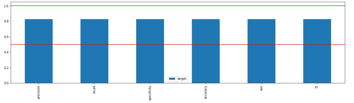

特定の列にわたってメトリックの不均衡を特定します

 _ = xai . metrics_plot (
    y_test , 
    probabilities , 
    df = x_test_display , 
    cross_cols = [ "gender" ],
    categorical_cols = categorical_cols )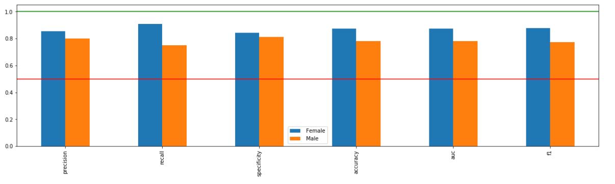

複数の列にわたってメトリックの不均衡を特定します

 _ = xai . metrics_plot (
    y_test , 
    probabilities , 
    df = x_test_display , 
    cross_cols = [ "gender" , "ethnicity" ],
    categorical_cols = categorical_cols )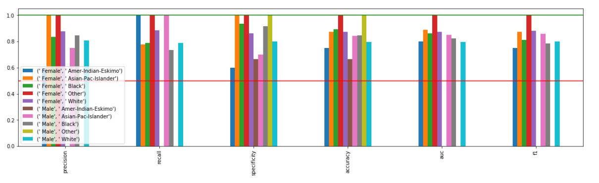

混乱マトリックスを描きます

 xai . confusion_matrix_plot ( y_test , pred )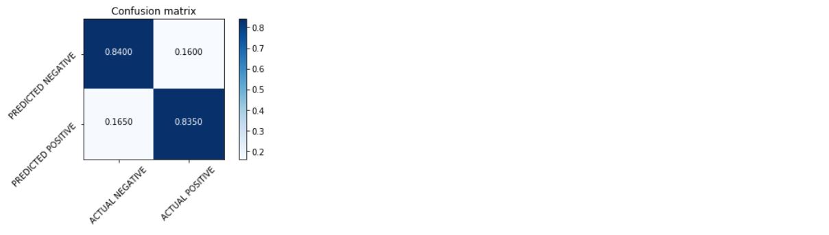

すべてのテストデータに対してROC曲線を視覚化します

 _ = xai . roc_plot ( y_test , probabilities )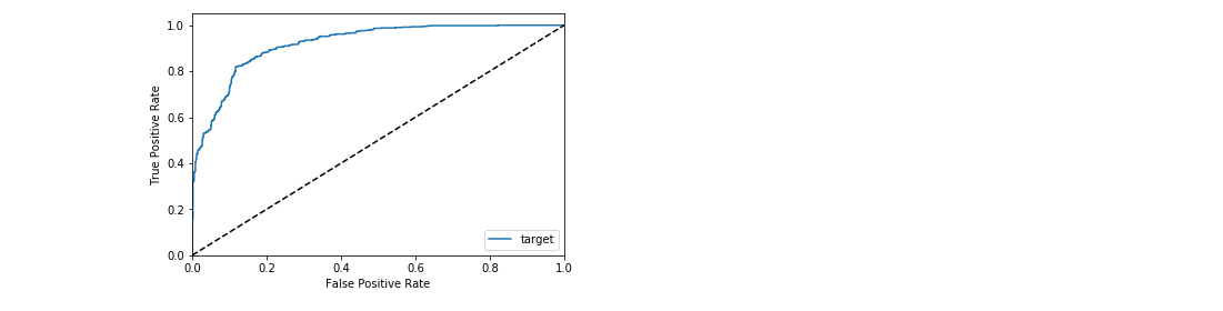

保護された列によってグループ化されたROC曲線を視覚化します

 protected = [ "gender" , "ethnicity" , "age" ]
_ = [ xai . roc_plot (
    y_test , 
    probabilities , 
    df = x_test_display , 
    cross_cols = [ p ],
    categorical_cols = categorical_cols ) for p in protected ]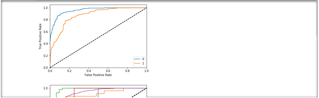

確率バケットによってグループ化された精度を視覚化します

 d = xai . smile_imbalance (
    y_test , 
    probabilities )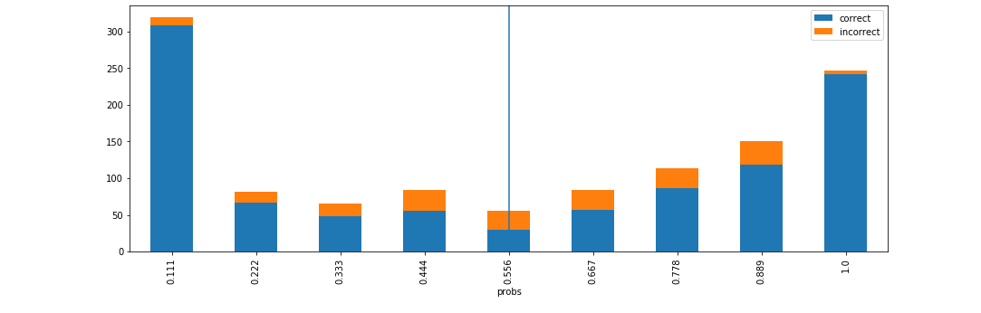

確率バケットによってグループ化された統計メトリックを視覚化します

 d = xai . smile_imbalance (
    y_test , 
    probabilities ,
    display_breakdown = True )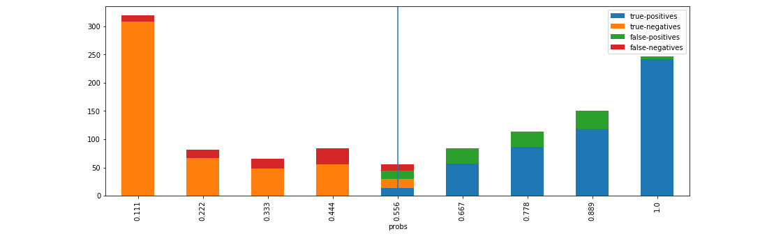

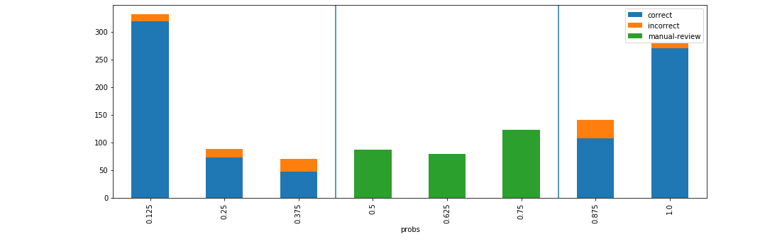
確率のしきい値に関する手動レビューを追加することの利点を視覚化します

 d = xai . smile_imbalance (
    y_test , 
    probabilities ,
    bins = 9 ,
    threshold = 0.75 ,
    manual_review = 0.375 ,
    display_breakdown = False )