named_entity_recognition
1.0.0
This project attempts to solve the problem of Chinese naming entity recognition using a variety of different models (including HMM, CRF, Bi-LSTM, Bi-LSTM+CRF). The data set uses the resume data collected in the paper ACL 2018 Chinese NER using Lattice LSTM. The format of the data is as follows. Each line of it is composed of a word and its corresponding annotation. The annotation set is BIOES and the sentences are separated by a blank line.
美	B-LOC
国	E-LOC
的	O
华	B-PER
莱	I-PER
士	E-PER

我	O
跟	O
他	O
谈	O
笑	O
风	O
生	O
This dataset is located in the ResumeNER folder in the project directory.
Here are four different models and the accuracy of the prediction results of these four models (taking the best):
| HMM | CRF | BiLSTM | BiLSTM+CRF | Ensemble | |
|---|---|---|---|---|---|
| Recall rate | 91.22% | 95.43% | 95.32% | 95.72% | 95.65% |
| Accuracy | 91.49% | 95.43% | 95.37% | 95.74% | 95.69% |
| F1 score | 91.30% | 95.42% | 95.32% | 95.70% | 95.64% |
The last column of Ensemble combines the prediction results of these four models and uses the "voting" method to obtain the final prediction results.
(Ensemble's three indicators are not as good as BiLSTM+CRF. It can be said that in the Ensemble process, it was the other three models that dragged BiLSTM+CRF)
For specific output, you can view the output.txt file.
First install the dependencies:
pip3 install -r requirement.txt
After installation, use it directly
python3 main.py
You can train and evaluate the model. The evaluation model will print out the model's accuracy, recall, F1 score value and confusion matrix. If you want to modify the relevant model parameters or training parameters, you can set it in the ./models/config.py file.
After training, if you want to load and evaluate the model, run the following command:
python3 test.pyHere is a brief introduction to these models (github web page does not support mathematical formulas very well, and the parts involved in formulas cannot be displayed normally. My blog has a more detailed introduction to these models and code):
The hidden Markov model describes the process of randomly generating unobservable state random sequences from a hidden Markov chain, and then generating an observation from each state to generate an observation random sequence (Li Hang Statistical Learning Method). The Hidden Markov model is determined by the initial state distribution, the state transition probability matrix, and the observed probability matrix.
Naming entity recognition can essentially be regarded as a sequence labeling problem. When using HMM to solve the sequence labeling problem of named entity recognition, what we can observe is the sequence composed of words (observation sequence), and what we cannot observe is the label corresponding to each word (state sequence).
The initial state distribution is the initialization probability of each label, and the state transition probability matrix is the probability of transferring from a certain label to the next label (that is, if the label of the previous word is $tag_i$, the probability of the label of the next word being $tag_j$ is
Under a certain mark, the probability of generating a certain word.
The training process of the HMM model corresponds to the learning problems of the Hidden Markov model (Li Hang's statistical learning method),
In fact, it is to estimate the three elements of the model based on the training data based on the maximum likelihood method, namely the initial state distribution, state transition probability matrix and observation probability matrix mentioned above. After the model is trained, the model is used for decoding, that is, for a given observation sequence, it is to find its corresponding state sequence. Here is to find the corresponding annotation for each word in the sentence for a given sentence. For this decoding problem, we use the Viterbi algorithm.
For specific details, please check the models/hmm.py file.
There are two assumptions in the HMM model: one is that the output observation values are strictly independent, and the other is that the current state is only related to the previous state during the state transition. That is to say, in the scenario of naming entity recognition, HMM believes that each word in the observed sentence is independent of each other, and the label of the current moment is only related to the label of the previous moment. But in fact, naming entity recognition often requires more features, such as part of speech, word context, etc. At the same time, the label of the current moment should be associated with the label of the previous moment and the next moment. Due to the existence of these two assumptions, it is obvious that the HMM model is flawed in solving the problem of named entity recognition.
Conditional random fields can not only express the dependence between observations, but also represent the complex dependence between the current observation and the previous and subsequent states, which can effectively overcome the problems faced by the HMM model.
In order to establish a conditional random field, we first need to define a set of feature functions, each feature function in the set takes the annotation sequence as input and the extracted features as output. Assume that the function set is:
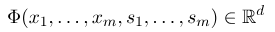
where $x=(x_1, ..., x_m)$ represents the observation sequence, and $s = (s_1, ......, s_m)$ represents the state sequence. The conditional random field then uses a logarithmic linear model to calculate the conditional probability of the state sequence under a given observation sequence:
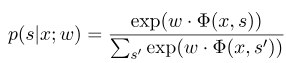
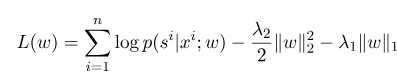
where $s^{'}$ is the sequence of all possible states, and $w$ is the parameter of the conditional random field model, which can be regarded as the weight of each feature function. The training of the CRF model is actually the estimation of the parameter $w$. Suppose we have $n$ marked data ${(x^i, s^i)}_{i=1}^n$,
Then the regularization form of its log-likelihood function is as follows:
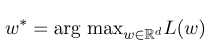
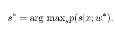
Then, the optimal parameter $w^*$ is:
After model training is completed, for the given observation sequence $x$, its corresponding optimal state sequence should be:
It is similar to HMM when decoding, and the Viterbi algorithm can also be used.
For specific details, please check the models/crf.py file.
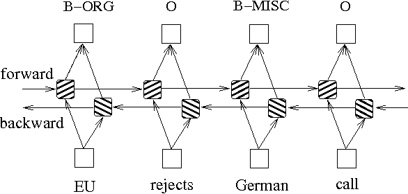
In addition to the above two methods based on probability graph models, LSTM is often used to solve the sequence labeling problem. Unlike HMM and CRF, LSTM relies on the strong nonlinear fitting ability of neural networks. During training, the samples are learned through complex nonlinear transformations in high-dimensional space, and then use this function to predict the annotation of each token for the specified sample. Below is a schematic diagram of sequence annotation using bidirectional LSTM (bidirectional can better capture the dependencies between sequences):
The sequence labeling model implementation based on bidirectional LSTM can view models/bilstm.py file.
The advantage of LSTM is that it can learn the dependence between observation sequences (input words) through bidirectional settings. During the training process, LSTM can automatically extract the characteristics of the observation sequence based on the target (such as identifying entities), but the disadvantage is that it cannot learn the relationship between state sequences (output labels). You should know that in the naming entity recognition task, there is a certain relationship between the labels. For example, a B label (representing the beginning of an entity) will not be followed by another B label. Therefore, when LSTM solves sequence labeling tasks such as NER, although it can eliminate complicated feature engineering, it also has the disadvantage of not being able to learn the labeling context.
On the contrary, the advantage of CRF is that it can model implicit states and learn the characteristics of state sequences, but its disadvantage is that it requires manual extraction of sequence features. So the general approach is to add another layer of CRF behind the LSTM to obtain the advantages of both.
For specific implementation, please see models/bilstm_crf.py
The problem of OOV (Out of vocabulary) needs to be handled in the HMM model, that is, some words in the test set are not in the training set. At this time, the probability of various states corresponding to OOV cannot be found through the observation probability matrix. To deal with this problem, the probability distribution of the state corresponding to OOV can be set to a uniform distribution.
When the three parameters of HMM (i.e., the state transition probability matrix, the observation probability matrix and the initial state probability matrix) are used for estimation using the supervised learning method, if some terms never appear, then the corresponding position of the term is 0. When decoding using the Viterbi algorithm, the calculation process needs to multiply these values. Then if there are terms with 0, the probability of the entire path will also become 0. In addition, multiple low probability multiplications during the decoding process are likely to cause underflow. In order to solve these two problems, we assign a very small number to those terms that have never appeared (such as 0.00000001). At the same time, when decoding, we map all three parameters of the model to the logarithmic space, which can not only avoid underflow, but also simplify the multiplication operation.
Before using training data and test data as input to the model in CRF, you need to use feature functions to extract features!
For Bi-LSTM+CRF model, you can refer to: Neural Architectures for Named Entity Recognition, and you can focus on the definition of the loss function in it. The calculation of loss functions in the code uses a method similar to dynamic programming, which is not easy to understand. Here we recommend looking at the following blogs:


