Torch Linguist
1.0.0
該項目是使用Pytorch構建語言模型的分步指南。它旨在對開發語言模型及其應用程序所涉及的過程進行全面的了解。
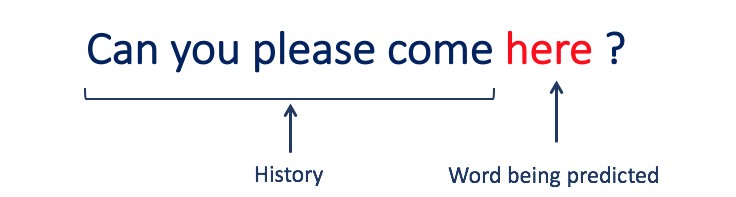
語言建模或LM是使用各種統計和概率技術來確定句子中出現的單詞序列的概率。語言模型分析文本數據的機構,為其單詞預測提供基礎。
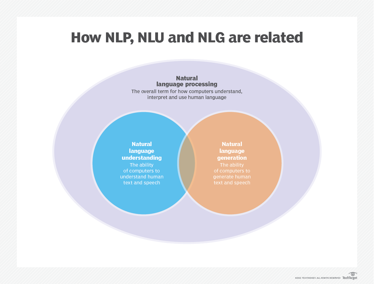
語言建模用於人工智能(AI),自然語言處理(NLP),自然語言理解(NLU)和自然語言生成(NLG)系統,尤其是執行文本生成,機器翻譯和問題答案的系統。
大型語言模型(LLMS)還使用語言建模。這些是高級語言模型,例如OpenAI的GPT-3和Google的Palm 2,它們處理數十億個培訓數據參數並生成文本輸出。
通常使用跨凝結和困惑等指標來評估語言模型的有效性,這些指標衡量了模型準確預測下一個單詞的能力(我將在步驟2中介紹它們)。幾個數據集,例如Wikitext-2,Wikitext-103,十億個單詞,Text8和C4等,通常用於評估語言模型。注意:在此項目中,我使用Wikitext-2。
LM的研究在文獻中受到了廣泛的關注,可以將其分為四個主要的發展階段:
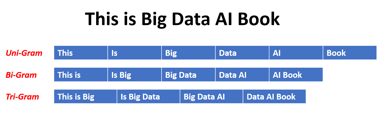
SLM是基於1990年代升起的統計學習方法而開發的。基本思想是基於馬爾可夫假設(例如,根據最新上下文預測下一個單詞)構建單詞預測模型。具有固定上下文長度n的SLM也稱為N-Gram語言模型,例如,Bigram和Trigram語言模型。 SLM已被廣泛應用於提高信息檢索(IR)和自然語言處理(NLP)的任務性能。但是,他們經常受到維度的詛咒:
由於需要估算指數次數的過渡概率,因此很難準確估計高階語言模型。因此,已經引入了專門設計的平滑策略,例如退縮估計和良好的估算,以減輕數據稀疏問題。
NLMS通過神經網絡,例如,多層感知器(MLP)和復發性神經網絡(RNN)來表徵單詞序列的概率。作為非凡的貢獻,是分佈式表示的概念。分佈式表示形式(也稱為嵌入式)的想法是,數據點的“含義”或“語義內容”分佈在多個維度上。例如,在NLP中,具有相似含義的單詞被映射到彼此接近的向量空間中的點。這種親密關係不是任意的,而是從單詞出現的上下文中學到的。這種與上下文相關的學習通常是通過神經網絡模型(例如Word2Vec或Glove )來實現的,該模型會處理大量文本以學習這些表示形式。
分佈式表示形式的關鍵優勢之一是它們捕獲細粒語義關係的能力。例如,在訓練有素的單詞嵌入空間中,同義詞將由近距離的向量表示,甚至可以使用這些向量對應於有意義的語義操作(例如,“ king” - “男人” - “男人” +“女人”的矢量進行算術操作,可能會導致矢量接近“ Queen”)。
分佈式表示的應用:
分佈式表示形式具有廣泛的應用,尤其是在涉及自然語言理解的任務中。它們用於:
單詞相似性:測量單詞之間的語義相似性。
文本分類:將文檔分類為預定義的類。
機器翻譯:將文本從一種語言轉換為另一種語言。
信息檢索:查找有關查詢的相關文檔。
情感分析:確定文本中表達的情感。
此外,分佈式表示不限於文本數據。它們還可以應用於其他類型的數據,例如圖像,其中深度學習模型學會將圖像表示為捕獲視覺特徵和語義的高維向量。
因果語言模型(也稱為自回歸模型)通過以前單詞的順序預測下一個單詞來生成文本。這些模型經過訓練,以最大程度地利用變壓器體系結構等技術來最大程度地提高下一個單詞的可能性。在訓練過程中,該模型的輸入是整個序列,直到給定令牌,該模型的目標是預測下一個令牌。這種類型的模型對於諸如文本生成,完成和摘要等任務很有用。
蒙版語言模型(MLMS)旨在通過預測句子中的蒙版或丟失單詞來學習單詞的上下文表示。在訓練過程中,一部分輸入序列被隨機掩蓋,並訓練該模型以預測給定上下文的原始單詞。 MLMS使用諸如變形金剛之類的雙向體系結構來捕獲蒙版單詞和句子其餘部分之間的依賴關係。這些模型在諸如文本分類,命名實體識別和問題答案之類的任務中表現出色。
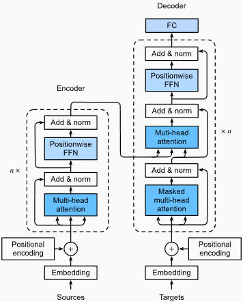
訓練序列到序列(SEQ2SEQ)模型以將輸入序列映射到輸出序列。它們由處理輸入序列的編碼器和生成輸出序列的解碼器組成。 SEQ2SEQ模型被廣泛用於機器翻譯,文本摘要和對話系統等任務。可以使用諸如復發神經網絡(RNN)或變形金剛等技術進行訓練。訓練目標是最大化給定輸入的正確輸出順序的可能性。
重要的是要注意,這些培訓方法不是相互排斥的,研究人員經常將它們結合起來或採用變化來實現特定目標。例如,諸如T5之類的模型結合了自回歸和掩蓋的語言模型培訓目標,以學習各種任務。
每種培訓方法都有其自己的優勢和劣勢,並且模型的選擇取決於特定的任務要求和可用培訓數據。
有關更多信息,請參閱“ Medium.com”網站上的語言模型培訓方法指南。
語言建模涉及構建可以生成或預測單詞或字符序列的模型。以下是一些通常用於語言建模的不同類型的模型:
在n-gram模型中,單詞的概率是根據訓練數據相對於其先前的n-1單詞在訓練數據中的出現而估計的。例如,在Trigram模型(n = 3)中,單詞的概率由緊接其之前的兩個單詞確定。這種方法假定單詞的概率僅取決於上一個固定數量的單詞,並且不考慮長期依賴性。
以下是n-grams的一些示例:
這是N-Gram語言模型的優點和缺點:
優點:
缺點:
這是在torchtext中使用n-grams的示例:
 import torchtext
from torchtext . data import get_tokenizer
from torchtext . data . utils import ngrams_iterator

tokenizer = get_tokenizer ( "basic_english" )
# Create a tokenizer object using the "basic_english" tokenizer provided by torchtext
# This tokenizer splits the input text into a list of tokens

tokens = tokenizer ( "I love to code in Python" )
# The result is a list of tokens, where each token represents a word or a punctuation mark

print ( list ( ngrams_iterator ( tokens , 3 )))

[ 'i' , 'love' , 'to' , 'code' , 'in' , 'python' , 'i love' , 'love to' , 'to code' , 'code in' , 'in python' , 'i love to' , 'love to code' , 'to code in' , 'code in python' ]筆記:
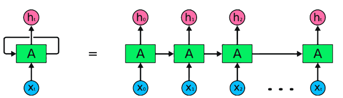
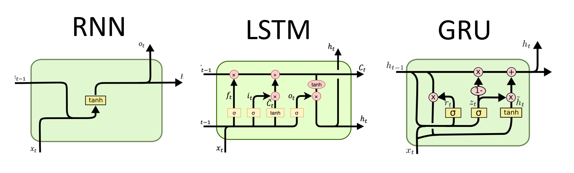
RNN是用於順序數據處理的神經網絡的基本類型。它們具有循環連接,允許信息從一個步驟傳遞到另一個步驟,從而使他們能夠跨時間捕獲依賴關係。但是,傳統的RNN遭受了消失/爆炸的梯度問題,並在長期依賴方面掙扎。
RNN的優勢:
RNN的缺點:
Pytorch代碼段用於定義Pytorch中的基本RNN:
 import torch
import torch . nn as nn

rnn = nn . RNN ( input_size = 10 , hidden_size = 20 , num_layers = 2 )
# input_size  – The number of expected features in the input x
# hidden_size – The number of features in the hidden state h
# num_layers  – Number of recurrent layers. E.g., setting num_layers=2 would mean stacking two RNNs together

# Create a randomly initialized input tensor
input = torch . randn ( 5 , 3 , 10 )  # (sequence length=5, batch size=3, input size=10)

# Create a randomly initialized hidden state tensor
h0 = torch . randn ( 2 , 3 , 20 )  # (num_layers=2, batch size=3, hidden size=20)

# Apply the RNN module to the input tensor and initial hidden state tensor
output , hn = rnn ( input , h0 )

print ( output . shape )  # torch.Size([5, 3, 20])
# (sequence length=5, batch size=3, hidden size=20)


print ( hn . shape )  # torch.Size([2, 3, 20])
# (num_layers=2, batch size=3, hidden size=20)LSTMS的優勢:
LSTMS的缺點:
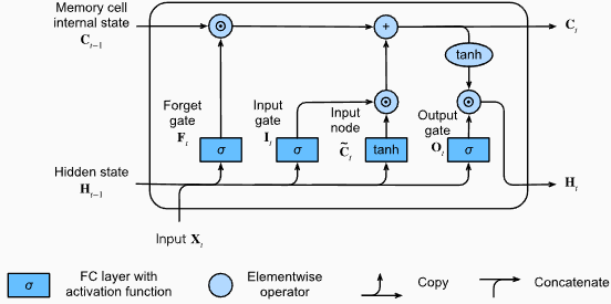
Pytorch代碼段用於定義Pytorch中的基本LSTM:
 import torch
import torch . nn as nn

input_size = 100
hidden_size = 64
num_layers = 2
batch_size = 1
seq_length = 10

lstm = nn . LSTM ( input_size , hidden_size , num_layers )
input_data = torch . randn ( seq_length , batch_size , input_size )
h0 = torch . zeros ( num_layers , batch_size , hidden_size )
c0 = torch . zeros ( num_layers , batch_size , hidden_size )

output , ( hn , cn ) = lstm ( input_data , ( h0 , c0 )) LSTM層的輸出形狀也將是[seq_length, batch_size, hidden_size] 。這意味著,對於序列中的每個輸入,將有一個相應的輸出隱藏狀態。在提供的示例中,輸出形狀為torch.Size([10, 1, 64]) ,表明LSTM應用於長度10的序列,批量大小為1,隱藏狀態大小為64。
現在,讓我們討論hn (隱藏狀態)張量。它的形狀為torch.Size([2, 1, 64]) 。第一個維度2表示LSTM中的層數。在這種情況下, num_layers參數設置為2,因此LSTM模型中有2層。第二維1,對應於批處理大小,在給定的示例中為1。最後,最後一個維度為64表示隱藏狀態的大小。
因此,遵循LSTM保留長期依賴性並減輕消失的梯度問題後, hn張量包含LSTM每一層的最終隱藏狀態。
有關更多信息,請參閱“深入深入學習”文檔中的長期短期記憶(LSTM)章節。
格魯斯的優勢:
格魯斯的缺點:
總體而言,LSTM和GRU模型克服了傳統RNN的某些局限性,尤其是在捕獲長期依賴方面。 LSTMS在保留上下文信息方面表現出色,而GRU提供了更有效的替代方案。 LSTM和GRU之間的選擇取決於任務的特定要求和可用的計算資源。
 import torch
import torch . nn as nn

input_size = 100
hidden_size = 64
num_layers = 2
batch_size = 1
seq_length = 10

gru = nn . GRU ( input_size , hidden_size , num_layers )
input_data = torch . randn ( seq_length , batch_size , input_size )
h0 = torch . zeros ( num_layers , batch_size , hidden_size )

output , hn = gru ( input_data , h0 ) GRU層的輸出形狀也將是[seq_length, batch_size, hidden_size] 。這意味著,對於序列中的每個輸入,將有一個相應的輸出隱藏狀態。在提供的示例中,輸出形狀為torch.Size([10, 1, 64]) ,表明GRU應用於長度10的序列,批量大小為1,隱藏狀態大小為64。
現在,讓我們討論hn (隱藏狀態)張量。它的形狀為torch.Size([2, 1, 64]) 。第一個維度為2表示GRU中的層數。在這種情況下, num_layers參數設置為2,因此GRU模型中有2層。第二維1,對應於批處理大小,在給定的示例中為1。最後,最後一個維度為64表示隱藏狀態的大小。
因此, hn張量在處理整個輸入序列後,遵循GRU捕獲和保留長序列的信息,同時減輕消失的梯度問題,在處理整個輸入序列後,包含GRU每一層的最終隱藏狀態。
有關更多信息,請參閱“深入深入學習”文檔中的封閉式複發單元(GRU)章節。
優點:
捕獲遠程依賴性:變形金剛通過使用自我注意的機制在序列中捕獲長距離依賴性方面表現出色。這使他們可以在做出預測時考慮輸入序列中的所有位置,從而更好地理解上下文並提高生成的文本質量。
並行處理:與復發模型不同,變壓器可以並行處理輸入序列,從而使其高效且減少訓練時間和推理時間。由於體系結構中沒有順序依賴性,因此可以進行這種並行化。
可擴展性:變壓器具有高度擴展性,可以有效處理大型輸入序列。他們可以處理任意長度的序列而無需截斷或填充,這對於涉及長文檔或句子的任務尤其有利。
上下文理解:變壓器可以通過參與輸入序列的相關部分來捕獲豐富的上下文信息。這使他們能夠理解單詞之間複雜的語言結構,語義關係和依賴性,從而導致更連貫和上下文適當的語言產生。
變壓器模型的缺點:
較高的計算要求:與N-Grams或傳統RNN(N-Grams或傳統的RNN)相比,變壓器通常需要大量的計算資源。使用大量數據集的培訓大型變壓器模型在計算上可能是昂貴且耗時的。
缺乏順序建模:當變壓器在捕獲全局依賴性方面表現出色時,它們可能在對嚴格的順序數據進行建模方面可能不那麼有效。如果輸入序列的順序至關重要,例如在涉及時間序列數據的任務中,傳統的RNN或卷積神經網絡(CNN)可能更合適。
注意機制的複雜性:變形金剛中的自我發揮機制為模型架構帶來了額外的複雜性。正確理解和實施注意力機制可能具有挑戰性,而與註意力相關的調整超參數可能是不平凡的。
數據要求:變壓器通常需要大量的培訓數據才能實現最佳性能。在大規模的語料庫中進行預處理,例如在驗證的變壓器模型(如GPT和BERT)的情況下,通常是有效地利用變形金剛的力量。
有關更多信息,請參閱“深入深入學習”文檔中的“變壓器架構”一章。
儘管有這些局限性,但變壓器模型徹底改變了自然語言處理和語言建模領域。他們捕獲長期依賴性和上下文理解的能力已在各種與語言有關的任務中顯著提高了最新技術的狀態,這使它們成為許多應用程序的重要選擇。
在語言建模的背景下,困惑性是一種量度,可以量化語言模型預測給定的測試集的能力,並具有較低的困惑表明更好的預測性能。用更簡單的術語,通過取測試集的反概率,然後通過單詞數將其歸一化來計算困惑。
困惑值越低,語言模型在預測測試集方面越好。最小化困惑與最大化概率相同
困惑性的公式作為測試集的反概率(按單詞數量標準化)如下:
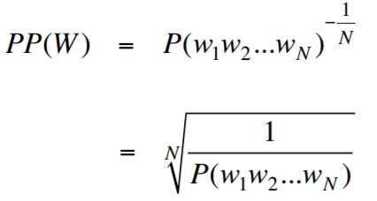
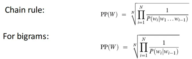
困惑性可以解釋為語言模型中分支因素的量度。分支因子代表了給定特定上下文或單詞序列的下一個單詞或令牌的平均數量。
語言的分支因素是可以遵循任何單詞的可能接下來單詞的數量。我們可以將困惑視為一種語言的加權平均分支係數。
使用嵌入層和LSTM代碼的語言建模是構建和培訓語言模型的強大工具。該代碼實現結合了自然語言處理中的兩個基本組件:嵌入層和長期記憶(LSTM)網絡。
嵌入層負責將文本數據轉換為分佈式表示形式,也稱為單詞嵌入。這些嵌入捕獲單詞的語義和句法屬性,從而使模型可以理解輸入文本的含義和上下文。嵌入層將輸入序列中的每個單詞映射到高維矢量,該向量是模型中後續層的輸入。
代碼實現中的LSTM層處理由嵌入層生成的單詞嵌入,捕獲序列信息並學習文本中的基本模式和結構。
通過組合嵌入層和LSTM網絡,該代碼可以構建可以生成連貫且上下文適當的文本的語言模型。使用這種方法構建的語言模型可以在大型文本數據集上進行培訓,並能夠生成現實且有意義的句子,使其成為各種自然語言處理任務的寶貴工具,例如文本生成,機器翻譯和情感分析。
此代碼實現為基於嵌入層和LSTM架構的構建語言模型提供了簡單,清晰和簡潔的基礎。它是有興趣探索和嘗試最先進的語言建模技術的研究人員,開發人員和愛好者的起點。
通過此代碼,您可以更深入地了解嵌入層和LSTM的方式以捕獲文本數據中的複雜模式和依賴項。有了這些知識,您可以進一步擴展代碼並探索高級技術,例如結合注意機製或變壓器體系結構,以增強語言模型的性能和能力。
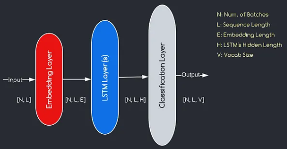
我們將構建的模型對應於上面提供的圖表,說明了三個關鍵組件:嵌入層,LSTM層和分類層。儘管我們已經熟悉LSTM和分類層的目標,但讓我們深入研究嵌入層的重要性。
嵌入層通過將表示為索引的每個單詞轉換為e維數的向量,在模型中起著至關重要的作用。該向量表示允許後續層從輸入中學習和提取有意義的信息。值得注意的是,使用索引或單速向量表示單詞可能不足,因為他們假設不同單詞之間沒有關係。
嵌入層進行的映射過程是在訓練過程中進行的學習過程。在這個訓練階段,該模型以捕獲語義和句法關係的方式將單詞與特定向量相關聯的能力,從而增強了模型對基本語言結構的理解。
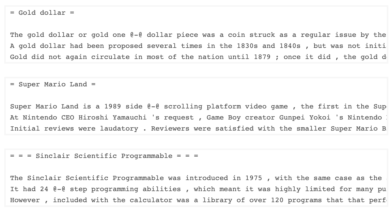
由Salesforce開發的Wkitext-103數據集包含超過1億個令牌,這些令牌從Wikipedia上的一系列經過驗證的商品和精選文章中提取出來。它具有267,340個獨特的令牌,在數據集中至少出現3次。由於它具有全長的Wikipedia文章,因此數據集非常適合可以使長期依賴性(例如語言建模)受益的任務。
Wikitext-2數據集是Wikitext-103數據集的一個小版本,因為它僅包含200萬個令牌。這個小數據集適用於測試您的語言模型。
該存儲庫包含用於對UTK數據集執行探索性數據分析的代碼,該代碼由按年齡,性別和種族分類的圖像組成。
要使用TorchText下載數據集,可以使用torchtext.datasets模塊。這是如何使用TorchText下載Wikitext-2數據集的示例:
 import torchtext
from torchtext . datasets import WikiText2
data_path = "data"
train_iter , valid_iter , test_iter = WikiText2 ( root = data_path ) 最初,我嘗試使用提供的代碼來加載Wikitext-2數據集,但遇到了URL的問題(https://s3.amazonaws.com/research.metamind.io/wikite.io/wikite.io/wikitext/wikitext-2-v1.zip)不起作用。為了克服這一點,我決定利用torchtext本庫並創建數據集加載程序的自定義實現。
由於原始URL無法正常工作,因此我從GitHub存儲庫下載了火車,驗證和測試數據集,並將其放置在'data/datasets/WikiText2'目錄中。
這是代碼的細分:
 import os
from typing import Union , Tuple

from torchdata . datapipes . iter import FileOpener , IterableWrapper
from torchtext . data . datasets_utils import _wrap_split_argument , _create_dataset_directory

DATA_DIR = "data"

NUM_LINES = {
    "train" : 36718 ,
    "valid" : 3760 ,
    "test" : 4358 ,
}

DATASET_NAME = "WikiText2"

_EXTRACTED_FILES = {
    "train" : "wiki.train.tokens" ,
    "test" : "wiki.test.tokens" ,
    "valid" : "wiki.valid.tokens" ,
}


def _filepath_fn ( root , split ):
    return os . path . join ( root , _EXTRACTED_FILES [ split ])


@ _create_dataset_directory ( dataset_name = DATASET_NAME )
@ _wrap_split_argument (( "train" , "valid" , "test" ))

def WikiText2 ( root : str , split : Union [ Tuple [ str ], str ]):
    url_dp = IterableWrapper ([ _filepath_fn ( DATA_DIR , split )])
    data_dp = FileOpener ( url_dp , encoding = "utf-8" ). readlines ( strip_newline = False , return_path = False ). shuffle (). set_shuffle ( False ). sharding_filter ()
return data_dp 要使用Wikitext-2數據集加載程序,只需導入Wikitext2函數,然後將其調用所需的數據拆分:
 train_data = WikiText2 ( root = "data/datasets/WikiText2" , split = "train" )
valid_data = WikiText2 ( root = "data/datasets/WikiText2" , split = "valid" )
test_data = WikiText2 ( root = "data/datasets/WikiText2" , split = "test" )該實現的靈感來自官方的TorchText數據集裝載機,並利用Torchdata和Torchtext庫提供了無縫有效的數據加載體驗。
在許多自然語言處理任務中,構建詞彙是至關重要的一步,因為它使您可以將單詞表示為可以在機器學習模型中使用的唯一標識符。該降價文檔演示瞭如何從一組培訓數據中構建詞彙並保存以備將來使用。
這是一個函數,封裝了構建和保存詞彙的過程:
 import torch
from torchtext . data . utils import get_tokenizer
from torchtext . vocab import build_vocab_from_iterator

def build_and_save_vocabulary ( train_iter , vocab_path = 'vocab.pt' , min_freq = 4 ):
    """
    Build a vocabulary from the training data iterator and save it to a file.

    Args:
        train_iter (iterator): An iterator over the training data.
        vocab_path (str, optional): The path to save the vocabulary file. Defaults to 'vocab.pt'.
        min_freq (int, optional): The minimum frequency of a word to be included in the vocabulary. Defaults to 4.

    Returns:
        torchtext.vocab.Vocab: The built vocabulary.
    """
    # Get the tokenizer
    tokenizer = get_tokenizer ( "basic_english" )

    # Build the vocabulary
    vocab = build_vocab_from_iterator ( map ( tokenizer , train_iter ), specials = [ '<unk>' ], min_freq = min_freq )

    # Set the default index to the unknown token
    vocab . set_default_index ( vocab [ '<unk>' ])

    # Save the vocabulary
    torch . save ( vocab , vocab_path )

    return vocab
這是您可以使用此功能的方法:
 # Assuming you have a training data iterator named `train_iter`
vocab = build_and_save_vocabulary ( train_iter , vocab_path = 'my_vocab.pt' )

# You can now use the vocabulary
print ( len ( vocab ))  # 23652
print ( vocab ([ 'ebi' , 'AI' . lower (), 'qwerty' ])) # [0, 1973, 0] build_and_save_vocabulary函數採用三個參數: train_iter (訓練數據上的迭代器), vocab_path (保存詞彙文件的路徑,默認為“ vocab.pt.pt'')和min_freq( min_freq (單詞的最小頻率都包含在vocabulary中的最小頻率,均為4)。basic_english Tokenizer,該函數在英語文本上執行基本令牌化。build_vocab_from_iterator函數來構建詞彙,傳遞訓練數據迭代器(後代化後)並指定'<unk>'特殊令牌和最小頻率閾值。'<unk>'令牌的ID,這意味著詞彙中未找到的任何單詞都會映射到未知的令牌上。要使用此功能,您需要擁有一個名為train_iter的培訓數據迭代器。然後,您可以調用build_and_save_vocabulary函數,通過train_iter並指定所需的詞彙文件路徑和最小頻率閾值。
該函數將構建詞彙,將其保存到指定的文件中,然後返回Vocab對象,然後您可以在下游任務中使用它們。
該代碼提供了一種分析Wikitext-2數據集中平均句子長度的方法。這是代碼的細分:
 import matplotlib . pyplot as plt

def compute_mean_sentence_length ( data_iter ):
    """
    Computes the mean sentence length for the given data iterator.

    Args:
        data_iter (iterable): An iterable of text data, where each element is a string representing a line of text.

    Returns:
        float: The mean sentence length.
    """
    total_sentence_count = 0
    total_sentence_length = 0

    for line in data_iter :
        sentences = line . split ( '.' )  # Split the line into individual sentences

        for sentence in sentences :
            tokens = sentence . strip (). split ()  # Tokenize the sentence
            sentence_length = len ( tokens )

            if sentence_length > 0 :
                total_sentence_count += 1
                total_sentence_length += sentence_length

    mean_sentence_length = total_sentence_length / total_sentence_count
    return mean_sentence_length

# Compute mean sentence length for each dataset
train_mean = compute_mean_sentence_length ( train_iter )
valid_mean = compute_mean_sentence_length ( valid_iter )
test_mean  = compute_mean_sentence_length ( test_iter )

# Plot the results
datasets = [ 'Train' , 'Valid' , 'Test' ]
means = [ train_mean , valid_mean , test_mean ]

plt . figure ( figsize = ( 6 , 4 ))
plt . bar ( datasets , means )
plt . xlabel ( 'Dataset' )
plt . ylabel ( 'Mean Sentence Length' )
plt . title ( 'Mean Sentence Length in Wikitext-2' )
plt . grid ( True )
plt . show ()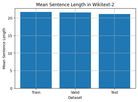
 from collections import Counter

# Compute word frequencies in the training dataset
freqs = Counter ()
for tokens in map ( tokenizer , train_iter ):
    freqs . update ( tokens )

# Find the 10 least common words
least_common_words = freqs . most_common ()[: - 11 : - 1 ]
print ( "Least Common Words:" )
for word , count in least_common_words :
    print ( f" { word } : { count } " )

# Find the 10 most common words
most_common_words = freqs . most_common ( 10 )
print ( " n Most Common Words:" )
for word , count in most_common_words :
print ( f" { word } : { count } " ) from collections import Counter
# Compute word frequencies in the training dataset
freqs = Counter ()
for tokens in map ( tokenizer , train_iter ):
freqs . update ( tokens )
# Count the number of words that repeat 3, 4, and 5 times
count_3 = count_4 = count_5 = 0
for word , freq in freqs . items ():
if freq == 3 :
count_3 += 1
elif freq == 4 :
count_4 += 1
elif freq == 5 :
count_5 += 1
print ( f"Number of words that appear 3 times: { count_3 } " ) # 5130
print ( f"Number of words that appear 4 times: { count_4 } " ) # 3243
print ( f"Number of words that appear 5 times: { count_5 } " ) # 2261 from collections import Counter
import matplotlib . pyplot as plt
# Compute the word lengths in the training dataset
word_lengths = []
for tokens in map ( tokenizer , train_iter ):
word_lengths . extend ( len ( word ) for word in tokens )
# Create a frequency distribution of word lengths
word_length_counts = Counter ( word_lengths )
# Plot the word length distribution
plt . figure ( figsize = ( 10 , 6 ))
plt . bar ( word_length_counts . keys (), word_length_counts . values ())
plt . xlabel ( "Word Length" )
plt . ylabel ( "Frequency" )
plt . title ( "Word Length Distribution in Wikitext-2 Dataset" )
plt . show ()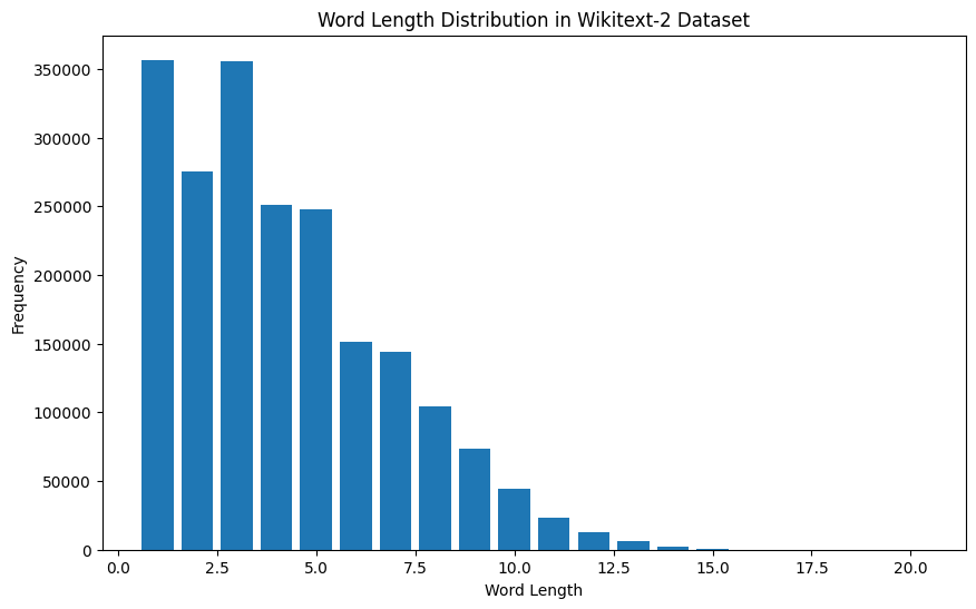
 import spacy
import en_core_web_sm

# Load the small English language model from SpaCy
nlp = spacy . load ( "en_core_web_sm" )

# Alternatively, you can use the en_core_web_sm module to load the model
nlp = en_core_web_sm . load ()

# Process the given sentence using the loaded language model
doc = nlp ( "This is a sentence." )

# Print the text and part-of-speech tag for each token in the sentence
print ([( w . text , w . pos_ ) for w in doc ])

# [('This', 'PRON'), ('is', 'AUX'), ('a', 'DET'), ('sentence', 'NOUN'), ('.', 'PUNCT')]
對於Wikitext-2數據集:
 import spacy

# Load the English language model
nlp = spacy . load ( "en_core_web_sm" )

# Perform POS tagging on the training dataset
pos_tags = []
for tokens in map ( tokenizer , train_iter ):
    doc = nlp ( " " . join ( tokens ))
    pos_tags . extend ([( token . text , token . pos_ ) for token in doc ])

# Count the frequency of each POS tag
pos_tag_counts = Counter ( tag for _ , tag in pos_tags )

# Print the most common POS tags
print ( "Most Common Part-of-Speech Tags:" )
for tag , count in pos_tag_counts . most_common ( 10 ):
    print ( f" { tag } : { count } " )

# Visualize the POS tag distribution
plt . figure ( figsize = ( 12 , 6 ))
plt . bar ( pos_tag_counts . keys (), pos_tag_counts . values ())
plt . xticks ( rotation = 90 )
plt . xlabel ( "Part-of-Speech Tag" )
plt . ylabel ( "Frequency" )
plt . title ( "Part-of-Speech Tag Distribution in Wikitext-2 Dataset" )
plt . show ()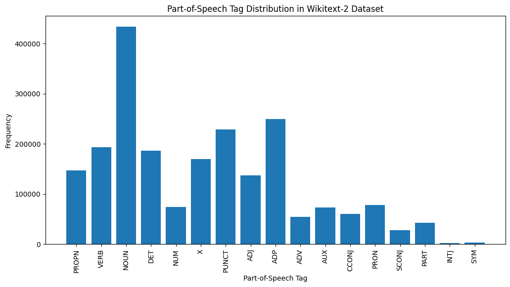
這是對提供的輸出中最常見的POS標籤的簡要說明:
名詞:名詞代表人,地方,事物或想法。
ADP :使用介詞和後置諸如介詞,用於表達單詞或短語之間的關係。
標點:標點符號,這對於分離和結構句子和文字至關重要。
動詞:動詞描述文本中的動作,狀態或事件。
DET :確定詞,例如文章(例如,“ the,” a,“”),提供了有關名詞的其他信息。
X :此標籤通常用於外語單詞,縮寫或其他不適合標準POS類別的特定語言令牌。
提示:代表人物,地點,組織或其他實體的特定名稱的專有名詞。
adj :形容詞修改或描述名詞和代詞。
pron :代詞代替名詞,使文本更簡潔,重複性較低。
數字:代表數量,日期或其他數值信息的數字。
POS標籤的這種分佈可以提供有關文本的語言特徵的見解,例如名詞的優勢,apositions的普遍性或適當名詞的使用,這可能有助於文本分類,信息提取或設式分析等任務。
 import spacy
import matplotlib . pyplot as plt

# Load the English language model
nlp = spacy . load ( "en_core_web_sm" )

# Perform NER on the training dataset
named_entities = []
for tokens in map ( tokenizer , train_iter ):
    doc = nlp ( " " . join ( tokens ))
    named_entities . extend ([( ent . text , ent . label_ ) for ent in doc . ents ])

# Count the frequency of each named entity type
ner_counts = Counter ( label for _ , label in named_entities )

# Print the most common named entity types
print ( "Most Common Named Entity Types:" )
for label , count in ner_counts . most_common ( 10 ):
    print ( f" { label } : { count } " )

# Visualize the named entity distribution
plt . figure ( figsize = ( 12 , 6 ))
plt . bar ( ner_counts . keys (), ner_counts . values ())
plt . xticks ( rotation = 90 )
plt . xlabel ( "Named Entity Type" )
plt . ylabel ( "Frequency" )
plt . title ( "Named Entity Distribution in Wikitext-2 Dataset" )
plt . show ()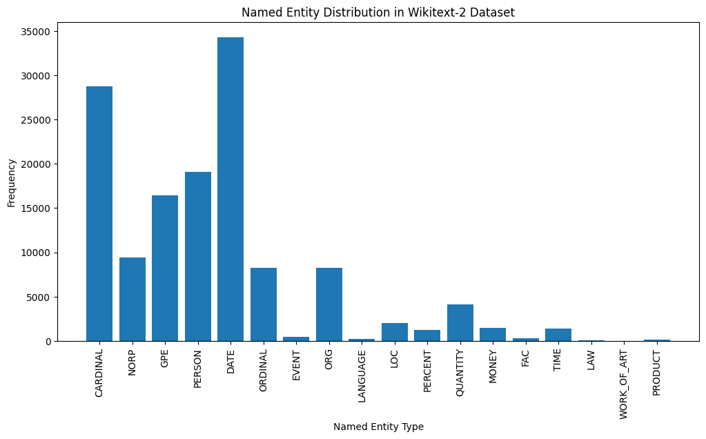
這是對輸出中最常見的命名實體類型的簡要說明:
日期:代表特定的日期,時間段或時間表達式,例如“ 2024年6月15日”或“去年”。
紅衣主教:包括數值,例如數量,年齡或測量值。
人:識別個人的名字。
GPE (地緣政治實體):該實體類型代表命名的地理位置,例如國家,城市或州。
NORP (國籍,宗教或政治團體):該實體類型包括基於國籍,宗教或政治意識形態的命名群體或隸屬關係。
序數:代表序數,例如“第一”,“第二”或“第三”。
組織(組織):公司,機構或其他有組織團體的姓名。
數量:包括非數量的數量,例如“幾個”或“幾個”。
LOC (位置):代表命名地理位置,例如大陸,區域或地形。
貨幣:標識貨幣價值,例如美元金額或貨幣名稱。
指定實體類型的這種分佈可以為文本的內容和重點提供寶貴的見解。例如,日期和基本實體的突出性可能提出一個涉及數字或時間信息的文本,而人,組織和GPE實體的流行率可以指示討論人,組織和地理位置的文本。
了解指定的實體分佈在各種應用程序中可能很有用,例如信息提取,問答和文本摘要,在此識別和分類命名的命名實體對於理解文本的上下文和內容至關重要。
 from wordcloud import WordCloud
import matplotlib . pyplot as plt

# Load the training dataset
with open ( "data/wiki.train.tokens" , "r" ) as f :
    train_text = f . read (). split ()

# Create a string from the entire training dataset
text = " " . join ( train_text )

# Generate the word cloud
wordcloud = WordCloud ( width = 800 , height = 400 , background_color = 'white' ). generate ( text )

# Plot the word cloud
plt . figure ( figsize = ( 12 , 8 ))
plt . imshow ( wordcloud , interpolation = 'bilinear' )
plt . axis ( 'off' )
plt . title ( 'Word Cloud for Wikitext-2 Training Dataset' )
plt . show ()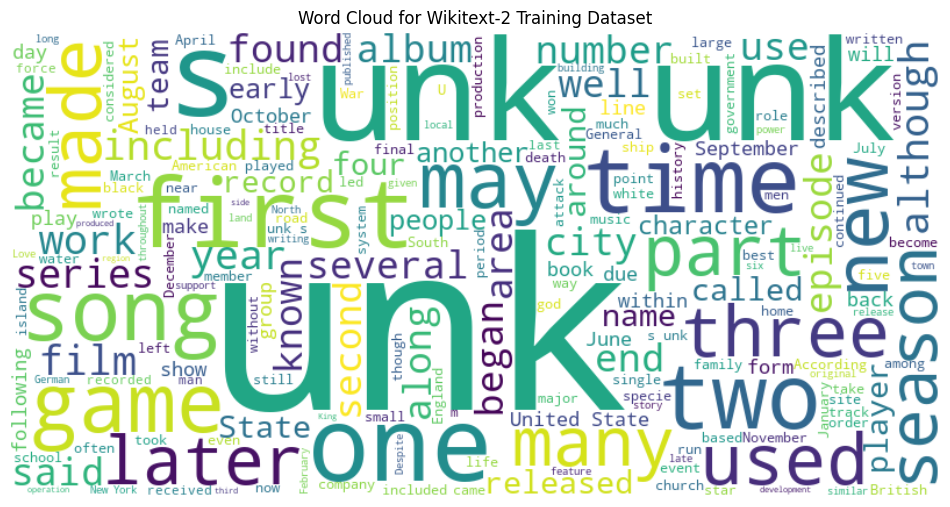
 from sentence_transformers import SentenceTransformer
from sklearn . cluster import KMeans
from collections import defaultdict
from wordcloud import WordCloud
import matplotlib . pyplot as plt

# Load the BERT-based sentence transformer model
model = SentenceTransformer ( 'bert-base-nli-mean-tokens' )

# Load the training dataset
with open ( "data/wiki.valid.tokens" , "r" ) as f :
    train_text = f . read (). split ()

# Compute the BERT embeddings for each unique word in the dataset
unique_words = set ( train_text )
word_embeddings = model . encode ( list ( unique_words ))

# Cluster the words using K-Means
num_clusters = 5
kmeans = KMeans ( n_clusters = num_clusters , random_state = 42 )
clusters = kmeans . fit_predict ( word_embeddings )

# Group the words by cluster
word_clusters = defaultdict ( list )
for i , word in enumerate ( unique_words ):
    word_clusters [ clusters [ i ]]. append ( word )

# Create a word cloud for each cluster
fig , axes = plt . subplots ( 1 , 5 , figsize = ( 14 , 12 ))
axes = axes . flatten ()

for cluster_id , cluster_words in word_clusters . items ():
    word_cloud = WordCloud ( width = 400 , height = 200 , background_color = 'white' ). generate ( ' ' . join ( cluster_words ))
    axes [ cluster_id ]. imshow ( word_cloud , interpolation = 'bilinear' )
    axes [ cluster_id ]. set_title ( f"Cluster { cluster_id } " )
    axes [ cluster_id ]. axis ( 'off' )

plt . subplots_adjust ( wspace = 0.4 , hspace = 0.6 )

plt . tight_layout ()
plt . show ()
兩種數據格式N x B x L和M x L通常用於語言建模任務中,尤其是在基於神經網絡的模型的背景下。
N x B x L格式:
N代表批處理數量。在這種情況下,數據集分為N較小的批次,這是提高培訓過程效率和穩定性的常見做法。B是批處理大小,它表示每個批次中樣本數(例如,句子,段落或文檔)的數量。L是每個批次中樣本的長度,通常對應於樣本中的令牌(單詞)數量。 M x L格式:
N x B x L格式相比,這種格式更簡單,更簡單。M等於N x B ,它代表數據集中樣本總數(例如,句子,段落或文檔)。L是每個樣品的長度,對應於樣品中的令牌數(單詞)。這兩種格式之間的選擇取決於您的語言建模任務的特定要求以及與您合作的神經網絡體系結構的功能。如果您要訓練基於神經網絡的語言模型,則通常首選N x B x L格式,因為它可以進行有效的基於批次的培訓,並可以導致更快的收斂性和更好的性能。但是,如果您的任務不涉及神經網絡或數據集相對較小,則M x L格式可能更合適。
 def prepare_language_model_data ( raw_text_iterator , sequence_length ):
    """
    Prepare PyTorch tensors for a language model.

    Args:
        raw_text_iterator (iterable): An iterator of raw text data.
        sequence_length (int): The length of the input and target sequences.

    Returns:
        tuple: A tuple containing two PyTorch tensors:
            - inputs (torch.Tensor): A tensor of input sequences.
            - targets (torch.Tensor): A tensor of target sequences.
    """
    # Convert the raw text iterator into a single PyTorch tensor
    data = torch . cat ([ torch . LongTensor ( vocab ( tokenizer ( line ))) for line in raw_text_iterator ])

    # Calculate the number of complete sequences that can be formed
    num_sequences = len ( data ) // sequence_length

    # Calculate the remainder of the data length divided by the sequence length
    remainder = len ( data ) % sequence_length

    # If the remainder is 0, add a single <unk> token to the end of the data tensor
    if remainder == 0 :
        unk_tokens = torch . LongTensor ([ vocab [ '<unk>' ]])
        data = torch . cat ([ data , unk_tokens ])

    # Extract the input and target sequences from the data tensor
    inputs = data [: num_sequences * sequence_length ]. reshape ( - 1 , sequence_length )
    targets = data [ 1 : num_sequences * sequence_length + 1 ]. reshape ( - 1 , sequence_length )

    print ( len ( inputs ), len ( targets ))
return inputs , targets sequence_length = 30
X_train , y_train = prepare_language_model_data ( train_iter , sequence_length )
X_valid , y_valid = prepare_language_model_data ( valid_iter , sequence_length )
X_test , y_test = prepare_language_model_data ( test_iter , sequence_length )
X_train . shape , y_train . shape , X_valid . shape , y_valid . shape , X_test . shape , y_test . shape
( torch . Size ([ 68333 , 30 ]),
torch . Size ([ 68333 , 30 ]),
torch . Size ([ 7147 , 30 ]),
torch . Size ([ 7147 , 30 ]),
torch . Size ([ 8061 , 30 ]),
torch . Size ([ 8061 , 30 ]))該代碼定義了用於使用語言模型數據的Pytorch Dataset集類別。 LanguageModelDataset類具有輸入和目標張量,並提供了訪問數據的必要方法。
 class LanguageModelDataset ( Dataset ):
    def __init__ ( self , inputs , targets ):
        self . inputs = inputs
        self . targets = targets

    def __len__ ( self ):
        return self . inputs . shape [ 0 ]

    def __getitem__ ( self , idx ):
return self . inputs [ idx ], self . targets [ idx ]LanguageModelDataset類可用如下:
 # Create the datasets
train_set = LanguageModelDataset ( X_train , y_train )
valid_set = LanguageModelDataset ( X_valid , y_valid )
test_set  = LanguageModelDataset ( X_test , y_test )

# Create data loaders (optional)
train_loader = DataLoader ( train_set , batch_size = 32 , shuffle = True )
valid_loader = DataLoader ( valid_set , batch_size = 32 )
test_loader  = DataLoader ( test_set , batch_size = 32 )

# Access the data
x_batch , y_batch = next ( iter ( train_loader ))
print ( f"Input batch shape: { x_batch . shape } " )  # Input batch shape: torch.Size([32, 30])
print ( f"Target batch shape: { y_batch . shape } " ) # Target batch shape: torch.Size([32, 30]) 該代碼定義了一種自定義的Pytorch語言模型,該模型允許您使用不同類型的單詞嵌入式,包括randomly初始化的嵌入,預訓練的GloVe嵌入式,預訓練的FastText嵌入式,通過簡單地指定創建模型實例時的embedding_type參數。
 import torch . nn as nn
from torchtext . vocab import GloVe , FastText


class LanguageModel ( nn . Module ):
    def __init__ ( self , vocab_size , embedding_dim ,
                 hidden_dim , num_layers , dropout_embd = 0.5 ,
                 dropout_rnn = 0.5 , embedding_type = 'random' ):

        super (). __init__ ()
        self . num_layers = num_layers
        self . hidden_dim = hidden_dim
        self . embedding_dim = embedding_dim
        self . embedding_type = embedding_type

        if embedding_type == 'random' :
            self . embedding = nn . Embedding ( vocab_size , embedding_dim )
            self . embedding . weight . data . uniform_ ( - 0.1 , 0.1 )

        elif embedding_type == 'glove' :
            self . glove = GloVe ( name = '6B' , dim = embedding_dim )
            self . embedding = nn . Embedding ( vocab_size , embedding_dim )
            self . embedding . weight . data . copy_ ( self . glove . vectors )
            self . embedding . weight . requires_grad = False

        elif embedding_type == 'fasttext' :
            self . glove = FastText ( language = 'en' )
            self . embedding = nn . Embedding ( vocab_size , embedding_dim )
            self . embedding . weight . data . copy_ ( self . fasttext . vectors )
            self . embedding . weight . requires_grad = False

        else :
            raise ValueError ( "Invalid embedding_type. Choose from 'random', 'glove', 'fasttext'." )

        self . dropout = nn . Dropout ( p = dropout_embd )
        self . lstm = nn . LSTM ( embedding_dim , hidden_dim , num_layers = num_layers ,
                           dropout = dropout_rnn , batch_first = True )
        self . fc = nn . Linear ( hidden_dim , vocab_size )

    def forward ( self , src ):
        embedding = self . dropout ( self . embedding ( src ))
        output , hidden = self . lstm ( embedding )
        prediction = self . fc ( output )
return prediction model = LanguageModel ( vocab_size = len ( vocab ),
embedding_dim = 300 ,
hidden_dim = 512 ,
num_layers = 2 ,
dropout_embd = 0.65 ,
dropout_rnn = 0.5 ,
embedding_type = 'glove' ) def num_trainable_params ( model ):
nums = sum ( p . numel () for p in model . parameters () if p . requires_grad ) / 1e6
return nums
# Calculate the number of trainable parameters in the embedding, LSTM, and fully connected layers of the LanguageModel instance 'model'
num_trainable_params ( model . embedding ) # (7.0956)
num_trainable_params ( model . lstm ) # (3.76832)
num_trainable_params ( model . fc ) # (12.133476)

