Torch Linguist
1.0.0
โครงการนี้เป็นคู่มือทีละขั้นตอนในการสร้างแบบจำลองภาษาโดยใช้ Pytorch มันมีจุดมุ่งหมายเพื่อให้ความเข้าใจที่ครอบคลุมเกี่ยวกับกระบวนการที่เกี่ยวข้องในการพัฒนารูปแบบภาษาและแอปพลิเคชัน
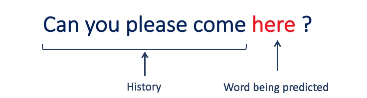
การสร้างแบบจำลองภาษาหรือ LM คือการใช้เทคนิคทางสถิติและความน่าจะเป็นต่างๆเพื่อกำหนดความน่าจะเป็นของลำดับคำที่เกิดขึ้นในประโยค แบบจำลองภาษาวิเคราะห์เนื้อหาของข้อมูลข้อความเพื่อให้พื้นฐานสำหรับการทำนายคำของพวกเขา
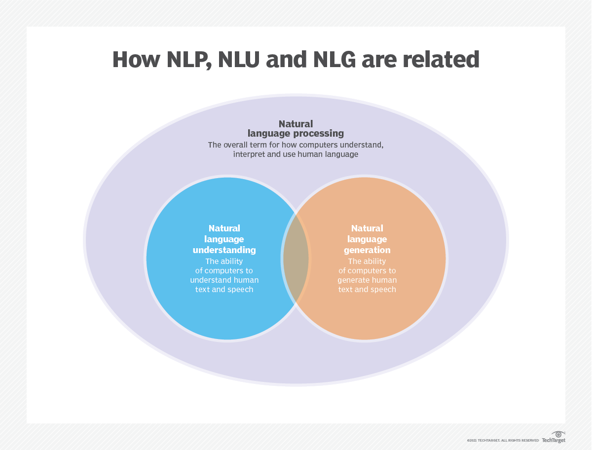
การสร้างแบบจำลองภาษาใช้ในปัญญาประดิษฐ์ (AI), การประมวลผลภาษาธรรมชาติ (NLP), การทำความเข้าใจภาษาธรรมชาติ (NLU), และระบบการสร้างภาษาธรรมชาติ (NLG) โดยเฉพาะอย่างยิ่งการสร้างการสร้างข้อความการแปลเครื่องและการตอบคำถาม
แบบจำลองภาษาขนาดใหญ่ (LLMS) ยังใช้การสร้างแบบจำลองภาษา เหล่านี้เป็นรูปแบบภาษาขั้นสูงเช่น GPT-3 ของ OpenAI และ Palm 2 ของ Google ซึ่งจัดการพารามิเตอร์ข้อมูลการฝึกอบรมหลายพันล้านและสร้างเอาต์พุตข้อความ
ประสิทธิภาพของแบบจำลองภาษามักจะถูกประเมินโดยใช้ตัวชี้วัดเช่น cross-entropy และ perplexity ซึ่งวัดความสามารถของแบบจำลองในการทำนายคำต่อไปอย่างแม่นยำ (ฉันจะครอบคลุมใน ขั้นตอนที่ 2 ) ชุดข้อมูลหลายชุดเช่น Wikitext-2, Wikitext-103, หนึ่งพันล้านคำ, text8 และ c4 ในหมู่คนอื่น ๆ มักใช้สำหรับการประเมินแบบจำลองภาษา หมายเหตุ : ในโครงการนี้ฉันใช้ Wikitext-2
การวิจัยของ LM ได้รับความสนใจอย่างกว้างขวางในวรรณคดีซึ่งสามารถแบ่งออกเป็นสี่ขั้นตอนการพัฒนาที่สำคัญ:
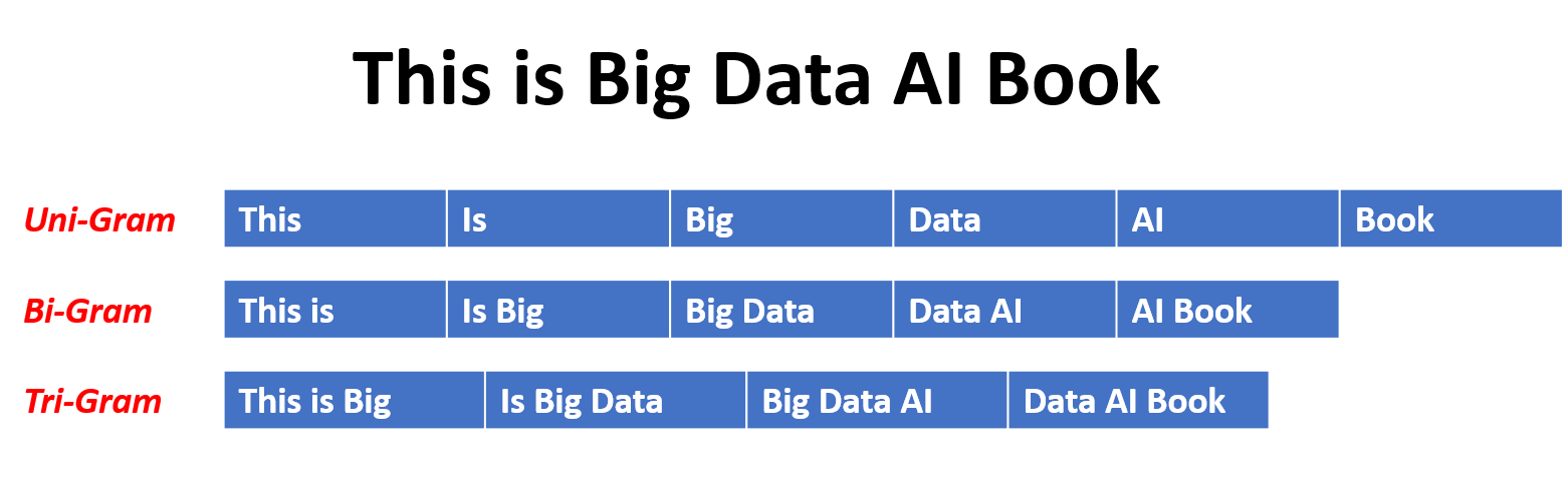
SLMS ได้รับการพัฒนาขึ้นอยู่กับวิธีการเรียนรู้ทางสถิติที่เพิ่มขึ้นในปี 1990 แนวคิดพื้นฐานคือการสร้างแบบจำลองการทำนายคำตาม สมมติฐานของมาร์คอฟ เช่นการทำนายคำต่อไปตามบริบทล่าสุด SLMS ที่มีความยาวบริบทคงที่ N เรียกอีกอย่างว่า โมเดลภาษา N-Gram เช่นโมเดลภาษา Bigram และ Trigram SLMS ได้รับการใช้อย่างกว้างขวางเพื่อเพิ่มประสิทธิภาพการทำงานในการดึงข้อมูล (IR) และการประมวลผลภาษาธรรมชาติ (NLP) อย่างไรก็ตามพวกเขามักจะประสบกับคำสาปของมิติ:
เป็นการยากที่จะประเมินแบบจำลองภาษาที่มีลำดับสูงอย่างถูกต้องเนื่องจากจำเป็นต้องประมาณความน่าจะเป็นของการเปลี่ยนแปลงจำนวนมาก ดังนั้นกลยุทธ์การปรับให้เรียบที่ออกแบบมาเป็นพิเศษเช่นการประมาณการกลับและการประมาณค่าที่ดีได้รับการแนะนำเพื่อบรรเทาปัญหาข้อมูล Sparsity
NLMS แสดงถึงความน่าจะเป็นของลำดับคำโดยเครือข่ายประสาทเช่น Multi-Layer Perceptron (MLP) และเครือข่ายประสาทที่เกิดขึ้นซ้ำ (RNNS) ในฐานะที่เป็นผลงานที่น่าทึ่งเป็นแนวคิดของ การเป็นตัวแทนแบบกระจาย การเป็นตัวแทนแบบกระจายหรือที่เรียกว่า Embeddings ความคิดคือ "ความหมาย" หรือ "เนื้อหาความหมาย" ของจุดข้อมูลจะถูกกระจายในหลายมิติ ตัวอย่างเช่นใน NLP คำที่มีความหมายคล้ายกันจะถูกแมปกับจุดในพื้นที่เวกเตอร์ที่อยู่ใกล้กัน ความใกล้ชิดนี้ไม่ได้เป็นไปตามอำเภอใจ แต่เรียนรู้จากบริบทที่คำที่ปรากฏ การเรียนรู้ที่ขึ้นกับบริบทนี้มักจะเกิดขึ้นได้จากโมเดลเครือข่ายประสาทเช่น Word2vec หรือ Glove ซึ่งประมวลผลข้อความขนาดใหญ่เพื่อเรียนรู้การเป็นตัวแทนเหล่านี้
หนึ่งในข้อได้เปรียบที่สำคัญของการเป็นตัวแทนแบบกระจายคือความสามารถในการจับความสัมพันธ์เชิงความหมายที่ดี ตัวอย่างเช่นในพื้นที่ฝังคำที่ผ่านการฝึกอบรมมาอย่างดีคำพ้องความหมายจะถูกแสดงโดยเวกเตอร์ที่อยู่ใกล้กันและเป็นไปได้ที่จะดำเนินการทางคณิตศาสตร์กับเวกเตอร์เหล่านี้ที่สอดคล้องกับการดำเนินการทางความหมายที่มีความหมาย (เช่น "ราชา" - "ผู้ชาย" + "ผู้หญิง" อาจส่งผลให้เวกเตอร์
แอปพลิเคชันของการเป็นตัวแทนแบบกระจาย:
การเป็นตัวแทนแบบกระจายมีแอพพลิเคชั่นที่หลากหลายโดยเฉพาะอย่างยิ่งในงานที่เกี่ยวข้องกับการทำความเข้าใจภาษาธรรมชาติ พวกเขาใช้สำหรับ:
ความคล้ายคลึงกันของคำ : การวัดความคล้ายคลึงกันระหว่างคำ
การจำแนกประเภทข้อความ : จัดหมวดหมู่เอกสารลงในคลาสที่กำหนดไว้ล่วงหน้า
การแปลของเครื่อง : การแปลข้อความจากภาษาหนึ่งไปอีกภาษาหนึ่ง
การดึงข้อมูล : การค้นหาเอกสารที่เกี่ยวข้องเพื่อตอบคำถาม
การวิเคราะห์ความเชื่อมั่น : การกำหนดความเชื่อมั่นที่แสดงเป็นชิ้นส่วนของข้อความ
นอกจากนี้การเป็นตัวแทนแบบกระจายไม่ จำกัด เฉพาะข้อมูลข้อความ พวกเขายังสามารถนำไปใช้กับข้อมูลประเภทอื่น ๆ เช่นภาพที่โมเดลการเรียนรู้ลึกเรียนรู้ที่จะแสดงภาพเป็นเวกเตอร์มิติสูงที่จับคุณสมบัติภาพและความหมาย
โมเดลภาษาเชิงสาเหตุหรือที่เรียกว่า โมเดล Autoregressive สร้างข้อความโดยทำนายคำถัดไปในลำดับที่ได้รับคำก่อนหน้านี้ โมเดลเหล่านี้ได้รับการฝึกฝนเพื่อเพิ่มโอกาสในการใช้คำต่อไปโดยใช้เทคนิคเช่นสถาปัตยกรรมหม้อแปลง ในระหว่างการฝึกอบรมอินพุตของโมเดลคือลำดับทั้งหมดจนถึงโทเค็นที่ได้รับและเป้าหมายของโมเดลคือการทำนายโทเค็นถัดไป โมเดลประเภทนี้มีประโยชน์สำหรับงานเช่น การสร้างข้อความ ความสมบูรณ์ และ การสรุป
แบบจำลองภาษาที่สวมหน้ากาก (MLMS) ได้รับการออกแบบมาเพื่อเรียนรู้การเป็นตัวแทนตามบริบทของคำโดยทำนาย คำที่สวมหน้ากากหรือคำที่หายไป ในประโยค ในระหว่างการฝึกอบรมส่วนหนึ่งของลำดับอินพุตจะถูกปกปิดแบบสุ่มและแบบจำลองได้รับการฝึกฝนให้ทำนายคำดั้งเดิมที่ได้รับบริบท MLMS ใช้สถาปัตยกรรมแบบสองทิศทางเช่นหม้อแปลงเพื่อจับการพึ่งพาระหว่างคำที่สวมหน้ากากและประโยคที่เหลือ โมเดลเหล่านี้เก่งในงานต่าง ๆ เช่น การจำแนกประเภทข้อความ การจดจำเอนทิตีชื่อ และ การตอบคำถาม
รุ่นลำดับต่อลำดับ (SEQ2SEQ) ได้รับการฝึกฝนให้แมปลำดับอินพุตกับลำดับเอาต์พุต พวกเขาประกอบด้วย ตัวเข้ารหัส ที่ประมวลผลลำดับอินพุตและ ตัวถอดรหัส ที่สร้างลำดับเอาต์พุต รุ่น SEQ2SEQ ถูกนำมาใช้กันอย่างแพร่หลายในงานเช่น การแปลด้วยเครื่อง การสรุปข้อความ และ ระบบการสนทนา พวกเขาสามารถได้รับการฝึกฝนโดยใช้เทคนิคต่าง ๆ เช่นเครือข่ายประสาท (RNNs) หรือหม้อแปลง วัตถุประสงค์การฝึกอบรมคือการเพิ่มโอกาสในการสร้างลำดับเอาต์พุตที่ถูกต้องให้สูงสุด
เป็นสิ่งสำคัญที่จะต้องทราบว่าวิธีการฝึกอบรมเหล่านี้ ไม่ได้เกิดขึ้นร่วมกัน และนักวิจัยมักจะรวมหรือใช้การเปลี่ยนแปลงเพื่อให้บรรลุเป้าหมายที่เฉพาะเจาะจง ตัวอย่างเช่นโมเดลเช่น T5 รวมวัตถุประสงค์การฝึกแบบโมเดลภาษาแบบอัตโนมัติและสวมหน้ากากเพื่อเรียนรู้งานที่หลากหลาย
วิธีการฝึกอบรมแต่ละวิธีมีจุดแข็งและจุดอ่อนของตัวเองและตัวเลือกของแบบจำลองขึ้นอยู่กับข้อกำหนดของงานเฉพาะและข้อมูลการฝึกอบรมที่มีอยู่
สำหรับข้อมูลเพิ่มเติมโปรดดูที่ A Guide to Language Model Training Approaches บทในเว็บไซต์ "medium.com"
การสร้างแบบจำลองภาษาเกี่ยวข้องกับการสร้างแบบจำลองที่สามารถสร้างหรือทำนายลำดับของคำหรืออักขระ นี่คือแบบจำลองบางประเภทที่ใช้กันทั่วไปสำหรับการสร้างแบบจำลองภาษา:
ในแบบจำลอง N-Gram ความน่าจะเป็นของคำนั้นถูกประเมินตามการเกิดขึ้นในข้อมูลการฝึกอบรมที่สัมพันธ์กับคำ N-1 ก่อนหน้านี้ ตัวอย่างเช่นในโมเดล trigram (n = 3) ความน่าจะเป็นของคำจะถูกกำหนดโดยสองคำที่นำหน้าทันที วิธีการนี้สันนิษฐานว่าความน่าจะเป็นของคำนั้นขึ้นอยู่กับจำนวนคำก่อนหน้านี้เท่านั้นและไม่ได้พิจารณาการพึ่งพาระยะยาว
นี่คือตัวอย่างของ N-Grams:
นี่คือข้อดีและข้อเสียของแบบจำลองภาษา N-Gram:
ข้อดี :
ข้อเสีย :
นี่คือตัวอย่างของการใช้ n-grams ใน Torchtext:
 import torchtext
from torchtext . data import get_tokenizer
from torchtext . data . utils import ngrams_iterator

tokenizer = get_tokenizer ( "basic_english" )
# Create a tokenizer object using the "basic_english" tokenizer provided by torchtext
# This tokenizer splits the input text into a list of tokens

tokens = tokenizer ( "I love to code in Python" )
# The result is a list of tokens, where each token represents a word or a punctuation mark

print ( list ( ngrams_iterator ( tokens , 3 )))

[ 'i' , 'love' , 'to' , 'code' , 'in' , 'python' , 'i love' , 'love to' , 'to code' , 'code in' , 'in python' , 'i love to' , 'love to code' , 'to code in' , 'code in python' ]
บันทึก :
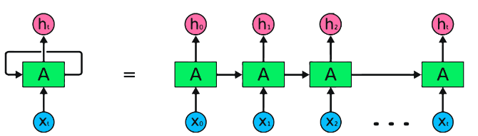
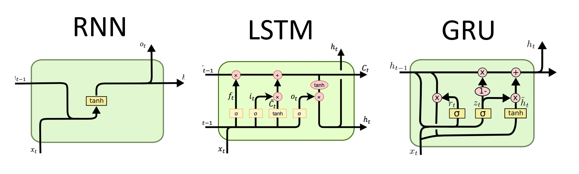
RNNs เป็นประเภทพื้นฐานของเครือข่ายประสาทสำหรับการประมวลผลข้อมูลตามลำดับ พวกเขามีการเชื่อมต่อซ้ำที่อนุญาตให้ส่งข้อมูลจากขั้นตอนหนึ่งไปยังอีกขั้นตอนต่อไปทำให้พวกเขาสามารถจับการพึ่งพาได้ตลอดเวลา อย่างไรก็ตาม RNN แบบดั้งเดิมได้รับผลกระทบจากปัญหาการไล่ระดับสีที่หายไป/ระเบิดและต่อสู้กับการพึ่งพาระยะยาว
ข้อดีของ RNNS :
ข้อเสียของ RNNS :
Pytorch รหัสตัวอย่างสำหรับการกำหนด rnn พื้นฐานใน pytorch:
 import torch
import torch . nn as nn

rnn = nn . RNN ( input_size = 10 , hidden_size = 20 , num_layers = 2 )
# input_size  – The number of expected features in the input x
# hidden_size – The number of features in the hidden state h
# num_layers  – Number of recurrent layers. E.g., setting num_layers=2 would mean stacking two RNNs together

# Create a randomly initialized input tensor
input = torch . randn ( 5 , 3 , 10 )  # (sequence length=5, batch size=3, input size=10)

# Create a randomly initialized hidden state tensor
h0 = torch . randn ( 2 , 3 , 20 )  # (num_layers=2, batch size=3, hidden size=20)

# Apply the RNN module to the input tensor and initial hidden state tensor
output , hn = rnn ( input , h0 )

print ( output . shape )  # torch.Size([5, 3, 20])
# (sequence length=5, batch size=3, hidden size=20)


print ( hn . shape )  # torch.Size([2, 3, 20])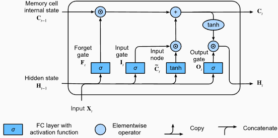
# (num_layers=2, batch size=3, hidden size=20)ข้อดีของ LSTMS :
ข้อเสียของ LSTMS :
Pytorch รหัสตัวอย่างสำหรับการกำหนด LSTM พื้นฐานใน pytorch:
 import torch
import torch . nn as nn

input_size = 100
hidden_size = 64
num_layers = 2
batch_size = 1
seq_length = 10

lstm = nn . LSTM ( input_size , hidden_size , num_layers )
input_data = torch . randn ( seq_length , batch_size , input_size )
h0 = torch . zeros ( num_layers , batch_size , hidden_size )
c0 = torch . zeros ( num_layers , batch_size , hidden_size )

output , ( hn , cn ) = lstm ( input_data , ( h0 , c0 ))
รูปร่างเอาต์พุตของเลเยอร์ LSTM จะเป็น [seq_length, batch_size, hidden_size] ซึ่งหมายความว่าสำหรับแต่ละอินพุตในลำดับจะมีสถานะที่ซ่อนอยู่ที่สอดคล้องกัน ในตัวอย่างที่ให้มารูปทรงเอาต์พุตคือ torch.Size([10, 1, 64]) ซึ่งบ่งชี้ว่า LSTM ถูกนำไปใช้กับลำดับความยาว 10 โดยมีขนาดแบทช์ 1 และขนาดสถานะที่ซ่อนอยู่ 64
ตอนนี้เรามาพูดคุยกันเรื่อง hn (สถานะที่ซ่อนอยู่) เทนเซอร์ รูปร่างของมันคือ torch.Size([2, 1, 64]) มิติแรก 2 แสดงถึงจำนวนเลเยอร์ใน LSTM ในกรณีนี้อาร์กิวเมนต์ num_layers ถูกตั้งค่าเป็น 2 ดังนั้นจึงมี 2 ชั้นในรุ่น LSTM มิติที่สอง 1 สอดคล้องกับขนาดแบทช์ซึ่งเป็น 1 ในตัวอย่างที่กำหนด ในที่สุดมิติสุดท้าย 64 แสดงถึงขนาดของสถานะที่ซ่อนอยู่
ดังนั้น hn Tensor จึงมีสถานะที่ซ่อนอยู่สุดท้ายสำหรับแต่ละเลเยอร์ของ LSTM หลังจากประมวลผลลำดับอินพุตทั้งหมดตามความสามารถของ LSTM ในการรักษาการพึ่งพาระยะยาวและลดปัญหาการไล่ระดับสีที่หายไป
สำหรับข้อมูลเพิ่มเติมโปรดดูบทหน่วยความจำระยะยาว (LSTM) ในเอกสาร "ดำน้ำสู่การเรียนรู้เชิงลึก"
ข้อดีของ GRUS :
ข้อเสียของ GRUS :
โดยรวมแล้วโมเดล LSTM และ GRU เอาชนะข้อ จำกัด บางประการของ RNN แบบดั้งเดิมโดยเฉพาะอย่างยิ่งในการจับการพึ่งพาระยะยาว LSTMS เก่งในการรักษาข้อมูลตามบริบทในขณะที่ GRUS เสนอทางเลือกที่มีประสิทธิภาพมากขึ้น ตัวเลือกระหว่าง LSTM และ GRU ขึ้นอยู่กับข้อกำหนดเฉพาะของงานและทรัพยากรการคำนวณที่มีอยู่
 import torch
import torch . nn as nn

input_size = 100
hidden_size = 64
num_layers = 2
batch_size = 1
seq_length = 10

gru = nn . GRU ( input_size , hidden_size , num_layers )
input_data = torch . randn ( seq_length , batch_size , input_size )
h0 = torch . zeros ( num_layers , batch_size , hidden_size )

output , hn = gru ( input_data , h0 )
รูปร่างเอาท์พุทของเลเยอร์ GRU จะเป็น [seq_length, batch_size, hidden_size] ซึ่งหมายความว่าสำหรับแต่ละอินพุตในลำดับจะมีสถานะที่ซ่อนอยู่ที่สอดคล้องกัน ในตัวอย่างที่ให้มารูปทรงเอาท์พุทคือ torch.Size([10, 1, 64]) ซึ่งบ่งชี้ว่า GRU ถูกนำไปใช้กับลำดับความยาว 10 โดยมีขนาดแบทช์ 1 และขนาดสถานะที่ซ่อนอยู่ 64
ตอนนี้เรามาพูดคุยกันเรื่อง hn (สถานะที่ซ่อนอยู่) เทนเซอร์ รูปร่างของมันคือ torch.Size([2, 1, 64]) มิติแรก 2 แสดงถึงจำนวนเลเยอร์ใน GRU ในกรณีนี้อาร์กิวเมนต์ num_layers ถูกตั้งค่าเป็น 2 ดังนั้นจึงมี 2 ชั้นในโมเดล GRU มิติที่สอง 1 สอดคล้องกับขนาดแบทช์ซึ่งเป็น 1 ในตัวอย่างที่กำหนด ในที่สุดมิติสุดท้าย 64 แสดงถึงขนาดของสถานะที่ซ่อนอยู่
ดังนั้น hn Tensor จึงมีสถานะที่ซ่อนอยู่สุดท้ายสำหรับแต่ละชั้นของ GRU หลังจากประมวลผลลำดับอินพุตทั้งหมดตามความสามารถของ GRU ในการจับและเก็บข้อมูลไว้ในลำดับที่ยาวนานในขณะที่บรรเทาปัญหาการไล่ระดับสีที่หายไป
สำหรับข้อมูลเพิ่มเติมโปรดดูบทที่มีการกำเริบของหน่วยที่มีรั้วรอบขอบชิด (GRU) ในเอกสาร "ดำน้ำสู่การเรียนรู้เชิงลึก"
ข้อดี :
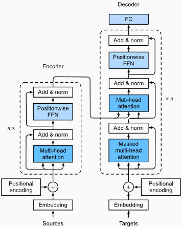
การจับการพึ่งพาระยะยาว: Transformers Excel ในการจับการพึ่งพาระยะยาวในลำดับโดยใช้กลไกการใส่ใจในตนเอง สิ่งนี้ช่วยให้พวกเขาพิจารณาตำแหน่งทั้งหมดในลำดับอินพุตเมื่อทำการคาดการณ์ช่วยให้เข้าใจบริบทที่ดีขึ้นและปรับปรุงคุณภาพของข้อความที่สร้างขึ้น
การประมวลผลแบบขนาน: ซึ่งแตกต่างจากแบบจำลองที่เกิดขึ้นอีกหม้อแปลงสามารถประมวลผลลำดับอินพุตแบบขนานทำให้มีประสิทธิภาพสูงและลดเวลาการฝึกอบรมและการอนุมาน การขนานนี้เป็นไปได้เนื่องจากไม่มีการพึ่งพาตามลำดับในสถาปัตยกรรม
ความสามารถในการปรับขนาด: หม้อแปลงสามารถปรับขนาดได้สูงและสามารถจัดการลำดับอินพุตขนาดใหญ่ได้อย่างมีประสิทธิภาพ พวกเขาสามารถประมวลผลลำดับของความยาวโดยพลการโดยไม่จำเป็นต้องตัดทอนหรือการขยายซึ่งเป็นประโยชน์อย่างยิ่งสำหรับงานที่เกี่ยวข้องกับเอกสารหรือประโยคยาว
ความเข้าใจในบริบท: Transformers สามารถบันทึกข้อมูลบริบทที่หลากหลายโดยเข้าร่วมกับส่วนที่เกี่ยวข้องของลำดับอินพุต สิ่งนี้ช่วยให้พวกเขาเข้าใจโครงสร้างทางภาษาที่ซับซ้อนความสัมพันธ์เชิงความหมายและการพึ่งพาระหว่างคำซึ่งส่งผลให้เกิดการสร้างภาษาที่สอดคล้องกันและเหมาะสมกับบริบทมากขึ้น
ข้อเสียของโมเดลหม้อแปลง :
ข้อกำหนดการคำนวณที่สูง: โดยทั่วไปแล้วหม้อแปลงต้องการทรัพยากรการคำนวณที่สำคัญเมื่อเทียบกับรุ่นที่ง่ายกว่าเช่น N-GRAM หรือ RNN แบบดั้งเดิม การฝึกอบรมแบบจำลองหม้อแปลงขนาดใหญ่ที่มีชุดข้อมูลที่กว้างขวางสามารถคำนวณได้ว่ามีราคาแพงและใช้เวลานาน
การขาดการสร้างแบบจำลองตามลำดับ: ในขณะที่ Transformers เก่งในการจับภาพการพึ่งพาทั่วโลก แต่อาจไม่ได้มีประสิทธิภาพในการสร้างแบบจำลองข้อมูลตามลำดับอย่างเคร่งครัด ในกรณีที่ลำดับของลำดับอินพุตมีความสำคัญเช่นในงานที่เกี่ยวข้องกับข้อมูลอนุกรมเวลา RNN แบบดั้งเดิมหรือเครือข่ายประสาท (CNNS) อาจเหมาะสมกว่า
ความซับซ้อนของกลไกความสนใจ: กลไกการดูแลตนเองในหม้อแปลงนำเสนอความซับซ้อนเพิ่มเติมให้กับสถาปัตยกรรมแบบจำลอง การทำความเข้าใจและการใช้กลไกความสนใจอย่างถูกต้องอาจเป็นเรื่องที่ท้าทายและการปรับพารามิเตอร์ไฮเปอร์พารามิเตอร์ที่เกี่ยวข้องกับความสนใจอาจไม่น่าสนใจ
ข้อกำหนดข้อมูล: หม้อแปลงมักจะต้องใช้ข้อมูลการฝึกอบรมจำนวนมากเพื่อให้ได้ประสิทธิภาพที่ดีที่สุด การเตรียมการใน corpora ขนาดใหญ่เช่นในกรณีของโมเดลหม้อแปลงที่ผ่านการฝึกอบรมเช่น GPT และ Bert เป็นเรื่องปกติที่จะใช้ประโยชน์จากพลังของหม้อแปลงอย่างมีประสิทธิภาพ
สำหรับข้อมูลเพิ่มเติมโปรดดูบทที่ Transformer Architecture ในเอกสาร "Dive Into Deep Learning"
แม้จะมีข้อ จำกัด เหล่านี้โมเดลหม้อแปลงได้ปฏิวัติสาขาการประมวลผลภาษาธรรมชาติและการสร้างแบบจำลองภาษา ความสามารถของพวกเขาในการจับการพึ่งพาระยะยาวและความเข้าใจตามบริบทได้พัฒนาสถานะของศิลปะอย่างมีนัยสำคัญในงานที่เกี่ยวข้องกับภาษาต่าง ๆ ทำให้พวกเขาเป็นตัวเลือกที่โดดเด่นสำหรับแอปพลิเคชันจำนวนมาก
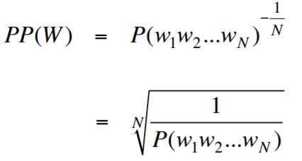
ความงุนงงในบริบทของการสร้างแบบจำลองภาษาเป็นมาตรการที่วัดปริมาณแบบจำลองภาษาที่ทำนายชุดทดสอบที่กำหนดได้ดีเพียงใด ในแง่ที่ง่ายกว่าความงุนงงจะถูกคำนวณโดยการใช้ความน่าจะเป็นแบบผกผันของชุดทดสอบแล้วปรับให้เป็นมาตรฐานด้วยจำนวนคำ
ยิ่งค่าความงงงวยยิ่งต่ำเท่าไหร่โมเดลภาษาก็จะดีกว่าในการทำนายชุดทดสอบ การลดความงุนงงให้น้อยที่สุดเหมือนกับการเพิ่มความน่าจะเป็นสูงสุด
สูตรสำหรับความงุนงงเป็นความน่าจะเป็นแบบผกผันของชุดทดสอบซึ่งถูกทำให้เป็นมาตรฐานด้วยจำนวนคำมีดังนี้:
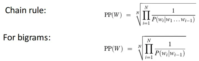
ความงุนงงสามารถตีความได้ว่าเป็นตัวชี้วัดของปัจจัยการแตกแขนงในรูปแบบภาษา ปัจจัยการแตกแขนงแสดงจำนวนเฉลี่ยของคำต่อไปหรือโทเค็นที่เป็นไปได้ที่ได้รับบริบทหรือลำดับของคำเฉพาะ
ปัจจัยการแตกแขนงของภาษาคือจำนวนคำต่อไปที่เป็นไปได้ที่สามารถทำตามคำใดก็ได้ เราสามารถนึกถึงความงุนงงว่าเป็นปัจจัยการแตกแขนงเฉลี่ยถ่วงน้ำหนักของภาษา
การสร้างแบบจำลองภาษาด้วยเลเยอร์การฝังและรหัส LSTM เป็นเครื่องมือที่ทรงพลังสำหรับการสร้างและการฝึกอบรมแบบจำลองภาษา การใช้รหัสนี้รวมองค์ประกอบพื้นฐานสองประการในการประมวลผลภาษาธรรมชาติ: เลเยอร์การฝัง และเครือข่ายหน่วย ความจำระยะสั้น (LSTM) ระยะยาว
เลเยอร์ฝังตัวมีหน้าที่ในการแปลงข้อมูลข้อความเป็นตัวแทนแบบกระจายหรือที่เรียกว่าคำว่า ฝังคำ การฝังตัวเหล่านี้จับคุณสมบัติความหมายและวากยสัมพันธ์ของคำช่วยให้แบบจำลองเข้าใจความหมายและบริบทของข้อความอินพุต เลเยอร์การฝังแผนที่แต่ละคำในลำดับอินพุตกับเวกเตอร์มิติสูงซึ่งทำหน้าที่เป็นอินพุตสำหรับเลเยอร์ที่ตามมาในโมเดล
เลเยอร์ LSTM ในการใช้งานรหัสจะประมวลผลคำที่ฝังอยู่โดยเลเยอร์การฝังการจับข้อมูลลำดับและเรียนรู้รูปแบบและโครงสร้างพื้นฐานในข้อความ
ด้วยการรวมเลเยอร์การฝังและเครือข่าย LSTM รหัสจะช่วยให้การสร้างแบบจำลองภาษาที่สามารถสร้างข้อความที่สอดคล้องกันและเหมาะสมตามบริบท แบบจำลองภาษาที่สร้างขึ้นโดยใช้วิธีการนี้สามารถได้รับการฝึกฝนในชุดข้อมูลข้อความขนาดใหญ่และมีความสามารถในการสร้างประโยคที่เป็นจริงและมีความหมายทำให้เป็นเครื่องมือที่มีค่าสำหรับงานการประมวลผลภาษาธรรมชาติที่หลากหลายเช่นการสร้างข้อความการแปลเครื่องและการวิเคราะห์ความเชื่อมั่น
การใช้รหัสนี้ให้รากฐานที่ง่ายชัดเจนและรัดกุมสำหรับการสร้างแบบจำลองภาษาตามสถาปัตยกรรมการฝังและสถาปัตยกรรม LSTM มันทำหน้าที่เป็นจุดเริ่มต้นสำหรับนักวิจัยนักพัฒนาและผู้ที่ชื่นชอบที่สนใจในการสำรวจและทดลองใช้เทคนิคการสร้างแบบจำลองภาษาที่ทันสมัย
ด้วยรหัสนี้คุณสามารถเข้าใจอย่างลึกซึ้งยิ่งขึ้นว่าการฝังเลเยอร์และ LSTMS ทำงานร่วมกันอย่างไรเพื่อจับรูปแบบที่ซับซ้อนและการพึ่งพาภายในข้อมูลข้อความ ด้วยความรู้นี้คุณสามารถขยายรหัสและสำรวจเทคนิคขั้นสูงเช่นการรวมกลไกความสนใจหรือสถาปัตยกรรมหม้อแปลงเพื่อเพิ่มประสิทธิภาพและความสามารถของแบบจำลองภาษาของคุณ
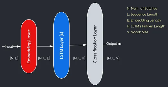
โมเดลที่เราจะสร้างสอดคล้องกับแผนภาพที่ให้ไว้ข้างต้นแสดงองค์ประกอบหลักสามประการ: เลเยอร์การฝัง, เลเยอร์ LSTM และเลเยอร์การจำแนกประเภท ในขณะที่วัตถุประสงค์ของเลเยอร์ LSTM และการจำแนกประเภทนั้นคุ้นเคยกับเราแล้วเรามาเจาะลึกลงไปในความสำคัญของเลเยอร์การฝัง
เลเยอร์การฝังมีบทบาทสำคัญในแบบจำลองโดยการเปลี่ยนแต่ละคำซึ่งแสดงเป็นดัชนีเป็นเวกเตอร์ของ มิติ E การเป็นตัวแทนเวกเตอร์นี้ช่วยให้เลเยอร์ที่ตามมาสามารถเรียนรู้และแยกข้อมูลที่มีความหมายออกจากอินพุต เป็นที่น่าสังเกตว่าการใช้ดัชนีหรือเวกเตอร์ที่ร้อนแรงหนึ่งครั้งเพื่อเป็นตัวแทนของคำอาจไม่เพียงพอเนื่องจากพวกเขาไม่มีความสัมพันธ์ระหว่างคำที่แตกต่างกัน
กระบวนการทำแผนที่ดำเนินการโดยเลเยอร์การฝังเป็นขั้นตอนการเรียนรู้ที่เกิดขึ้นระหว่างการฝึกอบรม ผ่านขั้นตอนการฝึกอบรมนี้โมเดลจะได้รับความสามารถในการเชื่อมโยงคำศัพท์กับเวกเตอร์เฉพาะในลักษณะที่จับความสัมพันธ์เชิงความหมายและวากยสัมพันธ์ซึ่งจะช่วยเพิ่มความเข้าใจของแบบจำลองเกี่ยวกับโครงสร้างภาษาพื้นฐาน
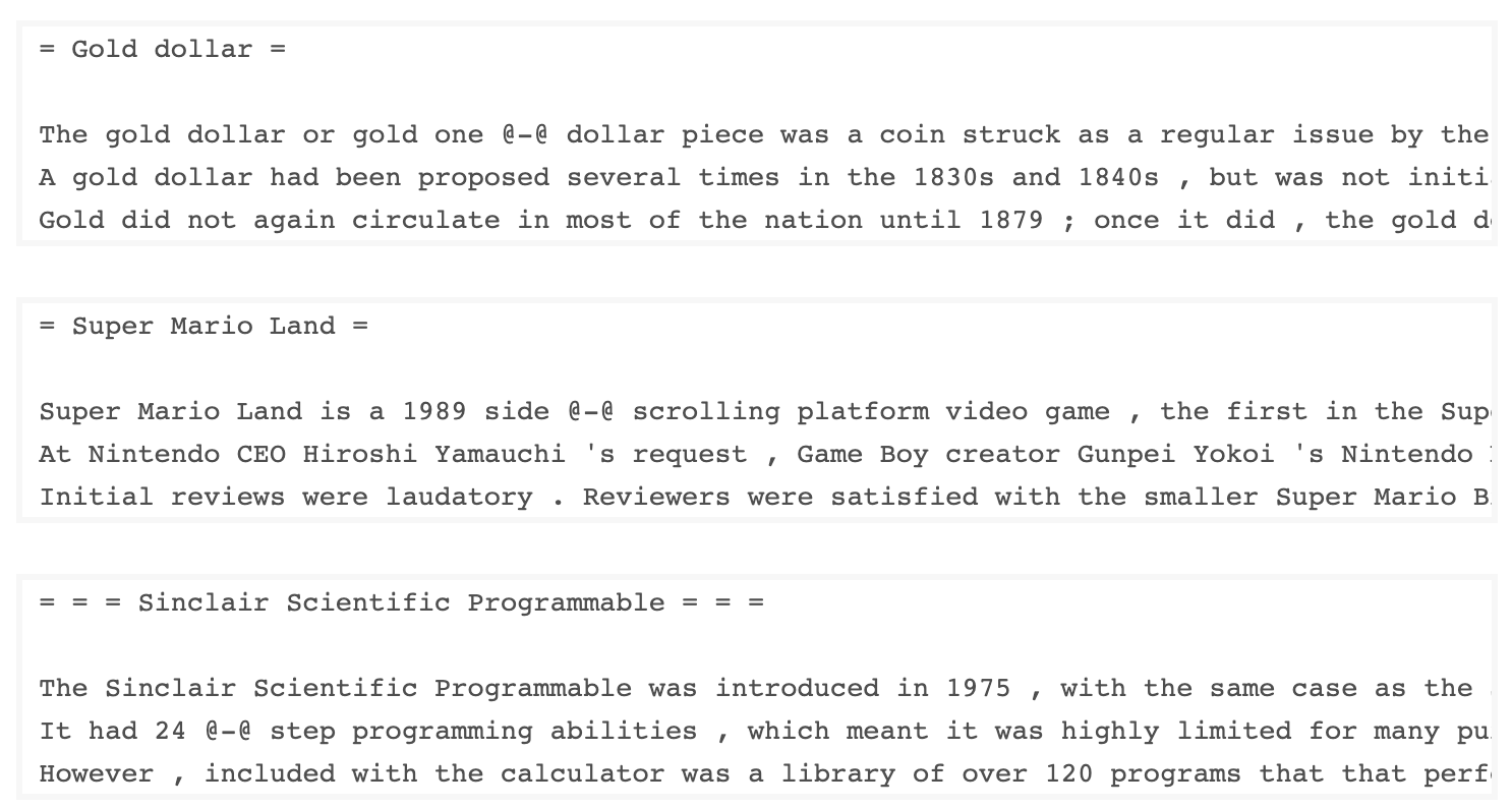
ชุดข้อมูล WKITEXT-103 ที่พัฒนาโดย Salesforce มีโทเค็นมากกว่า 100 ล้านโทที่สกัดจากชุดของบทความที่ดีและโดดเด่นเกี่ยวกับ Wikipedia มันมีโทเค็นที่ไม่ซ้ำกัน 267,340 ตัวที่ปรากฏอย่างน้อย 3 ครั้งในชุดข้อมูล เนื่องจากมีบทความ Wikipedia ที่มีความยาวเต็มรูปแบบชุดข้อมูลจึงเหมาะสำหรับงานที่สามารถรับประโยชน์จากการพึ่งพาระยะยาวเช่นการสร้างแบบจำลองภาษา
ชุดข้อมูล Wikitext-2 เป็นชุดข้อมูล Wikitext-103 รุ่นเล็กเนื่องจากมีโทเค็นเพียง 2 ล้านโท ชุดข้อมูลขนาดเล็กนี้เหมาะสำหรับการทดสอบรูปแบบภาษาของคุณ
ที่เก็บนี้มีรหัสสำหรับการวิเคราะห์ข้อมูลเชิงสำรวจในชุดข้อมูล UTK ซึ่งประกอบด้วยภาพที่จัดหมวดหมู่ตามอายุเพศและเชื้อชาติ
ในการดาวน์โหลดชุดข้อมูลโดยใช้ Torchtext คุณสามารถใช้โมดูล torchtext.datasets นี่คือตัวอย่างของวิธีการดาวน์โหลดชุดข้อมูล Wikitext-2 โดยใช้ TorchText:
 import torchtext
from torchtext . datasets import WikiText2
data_path = "data"
train_iter , valid_iter , test_iter = WikiText2 ( root = data_path )
เริ่มแรกฉันพยายามใช้รหัสที่ให้ไว้เพื่อโหลดชุดข้อมูล Wikitext-2 แต่พบปัญหากับ URL (https://s3.amazonaws.com/research.metamind.io/wikitext/wikitext-2-v1.zip) ไม่ทำงานสำหรับฉัน เพื่อเอาชนะสิ่งนี้ฉันตัดสินใจที่จะใช้ประโยชน์จากไลบรารี torchtext และสร้างการใช้งานที่กำหนดเองของตัวโหลดชุดข้อมูล
เนื่องจาก URL ดั้งเดิมไม่ทำงานฉันจึงดาวน์โหลดรถไฟการตรวจสอบและทดสอบชุดข้อมูลจากที่เก็บ GitHub และวางไว้ในไดเรกทอรี 'data/datasets/WikiText2'
นี่คือรายละเอียดของรหัส:
 import os
from typing import Union , Tuple

from torchdata . datapipes . iter import FileOpener , IterableWrapper
from torchtext . data . datasets_utils import _wrap_split_argument , _create_dataset_directory

DATA_DIR = "data"

NUM_LINES = {
    "train" : 36718 ,
    "valid" : 3760 ,
    "test" : 4358 ,
}

DATASET_NAME = "WikiText2"

_EXTRACTED_FILES = {
    "train" : "wiki.train.tokens" ,
    "test" : "wiki.test.tokens" ,
    "valid" : "wiki.valid.tokens" ,
}


def _filepath_fn ( root , split ):
    return os . path . join ( root , _EXTRACTED_FILES [ split ])


@ _create_dataset_directory ( dataset_name = DATASET_NAME )
@ _wrap_split_argument (( "train" , "valid" , "test" ))

def WikiText2 ( root : str , split : Union [ Tuple [ str ], str ]):
    url_dp = IterableWrapper ([ _filepath_fn ( DATA_DIR , split )])
    data_dp = FileOpener ( url_dp , encoding = "utf-8" ). readlines ( strip_newline = False , return_path = False ). shuffle (). set_shuffle ( False ). sharding_filter ()
return data_dp หากต้องการใช้ตัวโหลดชุดข้อมูล Wikitext-2 เพียงนำเข้าฟังก์ชั่น Wikitext2 และเรียกมันด้วยการแยกข้อมูลที่ต้องการ:
 train_data = WikiText2 ( root = "data/datasets/WikiText2" , split = "train" )
valid_data = WikiText2 ( root = "data/datasets/WikiText2" , split = "valid" )
test_data = WikiText2 ( root = "data/datasets/WikiText2" , split = "test" )การใช้งานนี้ได้รับแรงบันดาลใจจากชุดข้อมูล Torchtext อย่างเป็นทางการและใช้ประโยชน์จากไลบรารี TorchData และ Torchtext เพื่อมอบประสบการณ์การโหลดข้อมูลที่ราบรื่นและมีประสิทธิภาพ
การสร้างคำศัพท์เป็นขั้นตอนสำคัญในงานการประมวลผลภาษาธรรมชาติหลายอย่างเนื่องจากช่วยให้คุณแสดงคำเป็นตัวระบุที่ไม่ซ้ำกันที่สามารถใช้ในรูปแบบการเรียนรู้ของเครื่อง เอกสาร Markdown นี้แสดงให้เห็นถึงวิธีการสร้างคำศัพท์จากชุดข้อมูลการฝึกอบรมและบันทึกไว้สำหรับการใช้งานในอนาคต
นี่คือฟังก์ชั่นที่ห่อหุ้มกระบวนการสร้างและบันทึกคำศัพท์:
 import torch
from torchtext . data . utils import get_tokenizer
from torchtext . vocab import build_vocab_from_iterator

def build_and_save_vocabulary ( train_iter , vocab_path = 'vocab.pt' , min_freq = 4 ):
    """
    Build a vocabulary from the training data iterator and save it to a file.

    Args:
        train_iter (iterator): An iterator over the training data.
        vocab_path (str, optional): The path to save the vocabulary file. Defaults to 'vocab.pt'.
        min_freq (int, optional): The minimum frequency of a word to be included in the vocabulary. Defaults to 4.

    Returns:
        torchtext.vocab.Vocab: The built vocabulary.
    """
    # Get the tokenizer
    tokenizer = get_tokenizer ( "basic_english" )

    # Build the vocabulary
    vocab = build_vocab_from_iterator ( map ( tokenizer , train_iter ), specials = [ '<unk>' ], min_freq = min_freq )

    # Set the default index to the unknown token
    vocab . set_default_index ( vocab [ '<unk>' ])

    # Save the vocabulary
    torch . save ( vocab , vocab_path )

    return vocab
นี่คือวิธีที่คุณสามารถใช้ฟังก์ชั่นนี้:
 # Assuming you have a training data iterator named `train_iter`
vocab = build_and_save_vocabulary ( train_iter , vocab_path = 'my_vocab.pt' )

# You can now use the vocabulary
print ( len ( vocab ))  # 23652
print ( vocab ([ 'ebi' , 'AI' . lower (), 'qwerty' ])) # [0, 1973, 0] build_and_save_vocabulary ใช้เวลาสามข้อโต้แย้ง: train_iter (ตัววนซ้ำเหนือข้อมูลการฝึกอบรม), vocab_path (เส้นทางที่จะบันทึกไฟล์คำศัพท์โดยมีค่าเริ่มต้นของ 'Vocab.pt') และ min_freq (ความถี่ต่ำสุดของคำที่รวมอยู่ในคำศัพท์basic_english ซึ่งทำ tokenization ขั้นพื้นฐานในข้อความภาษาอังกฤษbuild_vocab_from_iterator ผ่านตัววนซ้ำข้อมูลการฝึกอบรม (หลังจาก tokenization) และระบุโทเค็นพิเศษ '<unk>' และเกณฑ์ความถี่ต่ำสุด'<unk>' ซึ่งหมายความว่าคำใด ๆ ที่ไม่พบในคำศัพท์จะถูกแมปกับโทเค็นที่ไม่รู้จัก ในการใช้ฟังก์ชั่นนี้คุณต้องมีตัววนซ้ำข้อมูลการฝึกอบรมชื่อ train_iter จากนั้นคุณสามารถเรียกฟังก์ชัน build_and_save_vocabulary ผ่าน train_iter และระบุเส้นทางไฟล์คำศัพท์ที่ต้องการและเกณฑ์ความถี่ขั้นต่ำ
ฟังก์ชั่นจะสร้างคำศัพท์บันทึกไปยังไฟล์ที่ระบุและส่งคืนวัตถุ Vocab ซึ่งคุณสามารถใช้ในงานดาวน์สตรีมของคุณ
รหัสนี้ให้วิธีการวิเคราะห์ความยาวประโยคเฉลี่ยในชุดข้อมูล Wikitext-2 นี่คือรายละเอียดของรหัส:
 import matplotlib . pyplot as plt

def compute_mean_sentence_length ( data_iter ):
    """
    Computes the mean sentence length for the given data iterator.

    Args:
        data_iter (iterable): An iterable of text data, where each element is a string representing a line of text.

    Returns:
        float: The mean sentence length.
    """
    total_sentence_count = 0
    total_sentence_length = 0

    for line in data_iter :
        sentences = line . split ( '.' )  # Split the line into individual sentences

        for sentence in sentences :
            tokens = sentence . strip (). split ()  # Tokenize the sentence
            sentence_length = len ( tokens )

            if sentence_length > 0 :
                total_sentence_count += 1
                total_sentence_length += sentence_length

    mean_sentence_length = total_sentence_length / total_sentence_count
    return mean_sentence_length

# Compute mean sentence length for each dataset
train_mean = compute_mean_sentence_length ( train_iter )
valid_mean = compute_mean_sentence_length ( valid_iter )
test_mean  = compute_mean_sentence_length ( test_iter )

# Plot the results
datasets = [ 'Train' , 'Valid' , 'Test' ]
means = [ train_mean , valid_mean , test_mean ]

plt . figure ( figsize = ( 6 , 4 ))
plt . bar ( datasets , means )
plt . xlabel ( 'Dataset' )
plt . ylabel ( 'Mean Sentence Length' )
plt . title ( 'Mean Sentence Length in Wikitext-2' )
plt . grid ( True )
plt . show ()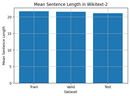
 from collections import Counter

# Compute word frequencies in the training dataset
freqs = Counter ()
for tokens in map ( tokenizer , train_iter ):
    freqs . update ( tokens )

# Find the 10 least common words
least_common_words = freqs . most_common ()[: - 11 : - 1 ]
print ( "Least Common Words:" )
for word , count in least_common_words :
    print ( f" { word } : { count } " )

# Find the 10 most common words
most_common_words = freqs . most_common ( 10 )
print ( " n Most Common Words:" )
for word , count in most_common_words :
print ( f" { word } : { count } " ) from collections import Counter
# Compute word frequencies in the training dataset
freqs = Counter ()
for tokens in map ( tokenizer , train_iter ):
freqs . update ( tokens )
# Count the number of words that repeat 3, 4, and 5 times
count_3 = count_4 = count_5 = 0
for word , freq in freqs . items ():
if freq == 3 :
count_3 += 1
elif freq == 4 :
count_4 += 1
elif freq == 5 :
count_5 += 1
print ( f"Number of words that appear 3 times: { count_3 } " ) # 5130
print ( f"Number of words that appear 4 times: { count_4 } " ) # 3243
print ( f"Number of words that appear 5 times: { count_5 } " ) # 2261 from collections import Counter
import matplotlib . pyplot as plt
# Compute the word lengths in the training dataset
word_lengths = []
for tokens in map ( tokenizer , train_iter ):
word_lengths . extend ( len ( word ) for word in tokens )
# Create a frequency distribution of word lengths
word_length_counts = Counter ( word_lengths )
# Plot the word length distribution
plt . figure ( figsize = ( 10 , 6 ))
plt . bar ( word_length_counts . keys (), word_length_counts . values ())
plt . xlabel ( "Word Length" )
plt . ylabel ( "Frequency" )
plt . title ( "Word Length Distribution in Wikitext-2 Dataset" )
plt . show ()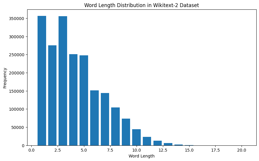
 import spacy
import en_core_web_sm

# Load the small English language model from SpaCy
nlp = spacy . load ( "en_core_web_sm" )

# Alternatively, you can use the en_core_web_sm module to load the model
nlp = en_core_web_sm . load ()

# Process the given sentence using the loaded language model
doc = nlp ( "This is a sentence." )

# Print the text and part-of-speech tag for each token in the sentence
print ([( w . text , w . pos_ ) for w in doc ])

# [('This', 'PRON'), ('is', 'AUX'), ('a', 'DET'), ('sentence', 'NOUN'), ('.', 'PUNCT')]
สำหรับชุดข้อมูล Wikitext-2:
 import spacy

# Load the English language model
nlp = spacy . load ( "en_core_web_sm" )

# Perform POS tagging on the training dataset
pos_tags = []
for tokens in map ( tokenizer , train_iter ):
    doc = nlp ( " " . join ( tokens ))
    pos_tags . extend ([( token . text , token . pos_ ) for token in doc ])

# Count the frequency of each POS tag
pos_tag_counts = Counter ( tag for _ , tag in pos_tags )

# Print the most common POS tags
print ( "Most Common Part-of-Speech Tags:" )
for tag , count in pos_tag_counts . most_common ( 10 ):
    print ( f" { tag } : { count } " )

# Visualize the POS tag distribution
plt . figure ( figsize = ( 12 , 6 ))
plt . bar ( pos_tag_counts . keys (), pos_tag_counts . values ())
plt . xticks ( rotation = 90 )
plt . xlabel ( "Part-of-Speech Tag" )
plt . ylabel ( "Frequency" )
plt . title ( "Part-of-Speech Tag Distribution in Wikitext-2 Dataset" )
plt . show ()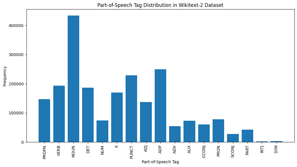
นี่คือคำอธิบายสั้น ๆ ของแท็ก POS ที่พบบ่อยที่สุดในเอาต์พุตที่ให้ไว้:
คำนาม : คำนามเป็นตัวแทนของผู้คนสถานที่สิ่งต่าง ๆ หรือความคิด
ADP : adpositions เช่นคำบุพบทและ postpositions ใช้เพื่อแสดงความสัมพันธ์ระหว่างคำหรือวลี
PURNT : เครื่องหมายวรรคตอนซึ่งจำเป็นสำหรับการแยกและจัดโครงสร้างประโยคและข้อความ
คำกริยา : คำกริยาอธิบายถึงการกระทำรัฐหรือเหตุการณ์ที่เกิดขึ้นในข้อความ
Det : ตัวกำหนดเช่นบทความ (เช่น "The," "A," "an") ให้ข้อมูลเพิ่มเติมเกี่ยวกับคำนาม
X : แท็กนี้มักจะใช้สำหรับคำต่างประเทศตัวย่อหรือโทเค็นเฉพาะภาษาอื่น ๆ ที่ไม่เหมาะสมกับหมวดหมู่ POS มาตรฐาน
Propn : คำนามที่เหมาะสมซึ่งเป็นตัวแทนชื่อเฉพาะของผู้คนสถานที่องค์กรหรือหน่วยงานอื่น ๆ
adj : คำคุณศัพท์แก้ไขหรืออธิบายคำนามและคำสรรพนาม
PRON : คำสรรพนามแทนคำนามทำให้ข้อความกระชับและซ้ำน้อยลง
NUM : ตัวเลขซึ่งแสดงถึงปริมาณวันที่หรือข้อมูลตัวเลขอื่น ๆ
การกระจายของแท็ก POS นี้สามารถให้ข้อมูลเชิงลึกเกี่ยวกับลักษณะทางภาษาของข้อความเช่นความเด่นของคำนามความชุกของ adpositions หรือการใช้คำนามที่เหมาะสมซึ่งจะเป็นประโยชน์ในงานเช่นการจำแนกข้อความการแยกข้อมูลหรือการวิเคราะห์ stylometric
 import spacy
import matplotlib . pyplot as plt

# Load the English language model
nlp = spacy . load ( "en_core_web_sm" )

# Perform NER on the training dataset
named_entities = []
for tokens in map ( tokenizer , train_iter ):
    doc = nlp ( " " . join ( tokens ))
    named_entities . extend ([( ent . text , ent . label_ ) for ent in doc . ents ])

# Count the frequency of each named entity type
ner_counts = Counter ( label for _ , label in named_entities )

# Print the most common named entity types
print ( "Most Common Named Entity Types:" )
for label , count in ner_counts . most_common ( 10 ):
    print ( f" { label } : { count } " )

# Visualize the named entity distribution
plt . figure ( figsize = ( 12 , 6 ))
plt . bar ( ner_counts . keys (), ner_counts . values ())
plt . xticks ( rotation = 90 )
plt . xlabel ( "Named Entity Type" )
plt . ylabel ( "Frequency" )
plt . title ( "Named Entity Distribution in Wikitext-2 Dataset" )
plt . show ()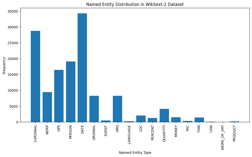
Here's a brief explanation of the most common named entity types in the output:
DATE : Represents specific dates, time periods, or temporal expressions, such as "June 15, 2024" or "last year".
CARDINAL : Includes numerical values, such as quantities, ages, or measurements.
PERSON : Identifies the names of individual people.
GPE (Geopolitical Entity): This entity type represents named geographical locations, such as countries, cities, or states.
NORP (Nationalities, Religious, or Political Groups): This entity type includes named groups or affiliations based on nationality, religion, or political ideology.
ORDINAL : Represents ordinal numbers, such as "first," "second," or "3rd".
ORG (Organization): The names of companies, institutions, or other organized groups.
QUANTITY : Includes non-numeric quantities, such as "a few" or "several".
LOC (Location): Represents named geographical locations, such as continents, regions, or landforms.
MONEY : Identifies monetary values, such as dollar amounts or currency names.
This distribution of named entity types can provide valuable insights into the content and focus of the text. For example, the prominence of DATE and CARDINAL entities may suggest a text that deals with numerical or temporal information, while the prevalence of PERSON, ORG, and GPE entities could indicate a text that discusses people, organizations, and geographical locations.
Understanding the named entity distribution can be useful in a variety of applications, such as information extraction, question answering, and text summarization, where identifying and categorizing key named entities is crucial for understanding the context and content of the text.
 from wordcloud import WordCloud
import matplotlib . pyplot as plt

# Load the training dataset
with open ( "data/wiki.train.tokens" , "r" ) as f :
    train_text = f . read (). split ()

# Create a string from the entire training dataset
text = " " . join ( train_text )

# Generate the word cloud
wordcloud = WordCloud ( width = 800 , height = 400 , background_color = 'white' ). generate ( text )

# Plot the word cloud
plt . figure ( figsize = ( 12 , 8 ))
plt . imshow ( wordcloud , interpolation = 'bilinear' )
plt . axis ( 'off' )
plt . title ( 'Word Cloud for Wikitext-2 Training Dataset' )
plt . show ()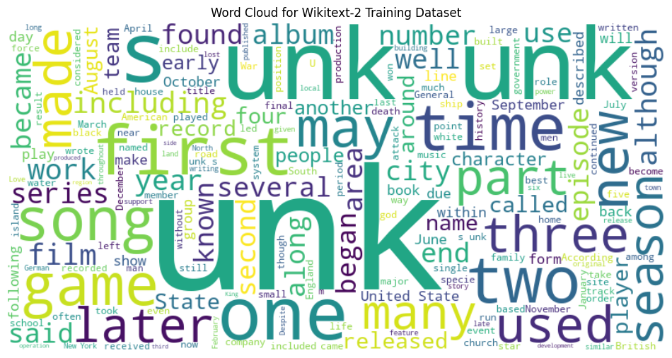
 from sentence_transformers import SentenceTransformer
from sklearn . cluster import KMeans
from collections import defaultdict
from wordcloud import WordCloud
import matplotlib . pyplot as plt

# Load the BERT-based sentence transformer model
model = SentenceTransformer ( 'bert-base-nli-mean-tokens' )

# Load the training dataset
with open ( "data/wiki.valid.tokens" , "r" ) as f :
    train_text = f . read (). split ()

# Compute the BERT embeddings for each unique word in the dataset
unique_words = set ( train_text )
word_embeddings = model . encode ( list ( unique_words ))

# Cluster the words using K-Means
num_clusters = 5
kmeans = KMeans ( n_clusters = num_clusters , random_state = 42 )
clusters = kmeans . fit_predict ( word_embeddings )

# Group the words by cluster
word_clusters = defaultdict ( list )
for i , word in enumerate ( unique_words ):
    word_clusters [ clusters [ i ]]. append ( word )

# Create a word cloud for each cluster
fig , axes = plt . subplots ( 1 , 5 , figsize = ( 14 , 12 ))
axes = axes . flatten ()

for cluster_id , cluster_words in word_clusters . items ():
    word_cloud = WordCloud ( width = 400 , height = 200 , background_color = 'white' ). generate ( ' ' . join ( cluster_words ))
    axes [ cluster_id ]. imshow ( word_cloud , interpolation = 'bilinear' )
    axes [ cluster_id ]. set_title ( f"Cluster { cluster_id } " )
    axes [ cluster_id ]. axis ( 'off' )

plt . subplots_adjust ( wspace = 0.4 , hspace = 0.6 )

plt . tight_layout ()
plt . show ()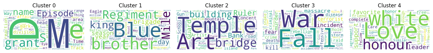
The two data formats, N x B x L and M x L , are commonly used in language modeling tasks, particularly in the context of neural network-based models.
N x B x L format:
N represents the number of batches. In this case, the dataset is divided into N smaller batches, which is a common practice to improve the efficiency and stability of the training process.B is the batch size, which represents the number of samples (eg, sentences, paragraphs, or documents) within each batch.L is the length of a sample within each batch, which typically corresponds to the number of tokens (words) in a sample. M x L format:
N x B x L format.M is equal to N x B , which represents the total number of samples (eg, sentences, paragraphs, or documents) in the dataset.L is the length of each sample, which corresponds to the number of tokens (words) in the sample. The choice between these two formats depends on the specific requirements of your language modeling task and the capabilities of the neural network architecture you're working with. If you're training a neural network-based language model, the N x B x L format is typically preferred, as it allows for efficient batch-based training and can lead to faster convergence and better performance. However, if your task doesn't involve neural networks or if the dataset is relatively small, the M x L format may be more suitable.
 def prepare_language_model_data ( raw_text_iterator , sequence_length ):
    """
    Prepare PyTorch tensors for a language model.

    Args:
        raw_text_iterator (iterable): An iterator of raw text data.
        sequence_length (int): The length of the input and target sequences.

    Returns:
        tuple: A tuple containing two PyTorch tensors:
            - inputs (torch.Tensor): A tensor of input sequences.
            - targets (torch.Tensor): A tensor of target sequences.
    """
    # Convert the raw text iterator into a single PyTorch tensor
    data = torch . cat ([ torch . LongTensor ( vocab ( tokenizer ( line ))) for line in raw_text_iterator ])

    # Calculate the number of complete sequences that can be formed
    num_sequences = len ( data ) // sequence_length

    # Calculate the remainder of the data length divided by the sequence length
    remainder = len ( data ) % sequence_length

    # If the remainder is 0, add a single <unk> token to the end of the data tensor
    if remainder == 0 :
        unk_tokens = torch . LongTensor ([ vocab [ '<unk>' ]])
        data = torch . cat ([ data , unk_tokens ])

    # Extract the input and target sequences from the data tensor
    inputs = data [: num_sequences * sequence_length ]. reshape ( - 1 , sequence_length )
    targets = data [ 1 : num_sequences * sequence_length + 1 ]. reshape ( - 1 , sequence_length )

    print ( len ( inputs ), len ( targets ))
return inputs , targets sequence_length = 30
X_train , y_train = prepare_language_model_data ( train_iter , sequence_length )
X_valid , y_valid = prepare_language_model_data ( valid_iter , sequence_length )
X_test , y_test = prepare_language_model_data ( test_iter , sequence_length )
X_train . shape , y_train . shape , X_valid . shape , y_valid . shape , X_test . shape , y_test . shape
( torch . Size ([ 68333 , 30 ]),
torch . Size ([ 68333 , 30 ]),
torch . Size ([ 7147 , 30 ]),
torch . Size ([ 7147 , 30 ]),
torch . Size ([ 8061 , 30 ]),
torch . Size ([ 8061 , 30 ])) This code defines a PyTorch Dataset class for working with language model data. The LanguageModelDataset class takes in input and target tensors and provides the necessary methods for accessing the data.
 class LanguageModelDataset ( Dataset ):
    def __init__ ( self , inputs , targets ):
        self . inputs = inputs
        self . targets = targets

    def __len__ ( self ):
        return self . inputs . shape [ 0 ]

    def __getitem__ ( self , idx ):
return self . inputs [ idx ], self . targets [ idx ] The LanguageModelDataset class can be used as follows:
 # Create the datasets
train_set = LanguageModelDataset ( X_train , y_train )
valid_set = LanguageModelDataset ( X_valid , y_valid )
test_set  = LanguageModelDataset ( X_test , y_test )

# Create data loaders (optional)
train_loader = DataLoader ( train_set , batch_size = 32 , shuffle = True )
valid_loader = DataLoader ( valid_set , batch_size = 32 )
test_loader  = DataLoader ( test_set , batch_size = 32 )

# Access the data
x_batch , y_batch = next ( iter ( train_loader ))
print ( f"Input batch shape: { x_batch . shape } " )  # Input batch shape: torch.Size([32, 30])
print ( f"Target batch shape: { y_batch . shape } " ) # Target batch shape: torch.Size([32, 30]) The code defines a custom PyTorch language model that allows you to use different types of word embeddings, including randomly initialized embeddings, pre-trained GloVe embeddings, pre-trained FastText embeddings, by simply specifying the embedding_type argument when creating the model instance.
 import torch . nn as nn
from torchtext . vocab import GloVe , FastText


class LanguageModel ( nn . Module ):
    def __init__ ( self , vocab_size , embedding_dim ,
                 hidden_dim , num_layers , dropout_embd = 0.5 ,
                 dropout_rnn = 0.5 , embedding_type = 'random' ):

        super (). __init__ ()
        self . num_layers = num_layers
        self . hidden_dim = hidden_dim
        self . embedding_dim = embedding_dim
        self . embedding_type = embedding_type

        if embedding_type == 'random' :
            self . embedding = nn . Embedding ( vocab_size , embedding_dim )
            self . embedding . weight . data . uniform_ ( - 0.1 , 0.1 )

        elif embedding_type == 'glove' :
            self . glove = GloVe ( name = '6B' , dim = embedding_dim )
            self . embedding = nn . Embedding ( vocab_size , embedding_dim )
            self . embedding . weight . data . copy_ ( self . glove . vectors )
            self . embedding . weight . requires_grad = False

        elif embedding_type == 'fasttext' :
            self . glove = FastText ( language = 'en' )
            self . embedding = nn . Embedding ( vocab_size , embedding_dim )
            self . embedding . weight . data . copy_ ( self . fasttext . vectors )
            self . embedding . weight . requires_grad = False

        else :
            raise ValueError ( "Invalid embedding_type. Choose from 'random', 'glove', 'fasttext'." )

        self . dropout = nn . Dropout ( p = dropout_embd )
        self . lstm = nn . LSTM ( embedding_dim , hidden_dim , num_layers = num_layers ,
                           dropout = dropout_rnn , batch_first = True )
        self . fc = nn . Linear ( hidden_dim , vocab_size )

    def forward ( self , src ):
        embedding = self . dropout ( self . embedding ( src ))
        output , hidden = self . lstm ( embedding )
        prediction = self . fc ( output )
return prediction model = LanguageModel ( vocab_size = len ( vocab ),
embedding_dim = 300 ,
hidden_dim = 512 ,
num_layers = 2 ,
dropout_embd = 0.65 ,
dropout_rnn = 0.5 ,
embedding_type = 'glove' ) def num_trainable_params ( model ):
nums = sum ( p . numel () for p in model . parameters () if p . requires_grad ) / 1e6
return nums
# Calculate the number of trainable parameters in the embedding, LSTM, and fully connected layers of the LanguageModel instance 'model'
num_trainable_params ( model . embedding ) # (7.0956)
num_trainable_params ( model . lstm ) # (3.76832)
num_trainable_params ( model . fc ) # (12.133476)

