Torch Linguist
1.0.0
This project is a step-by-step guide on building a language model using PyTorch. It aims to provide a comprehensive understanding of the process involved in developing a language model and its applications.
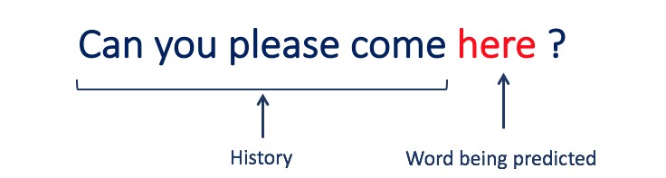
Language modeling, or LM, is the use of various statistical and probabilistic techniques to determine the probability of a given sequence of words occurring in a sentence. Language models analyze bodies of text data to provide a basis for their word predictions.
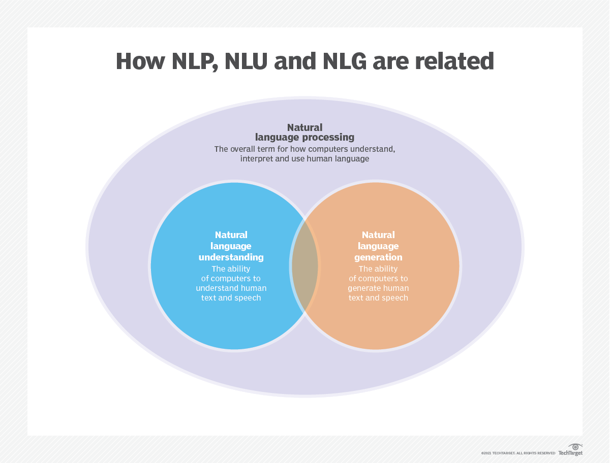
Language modeling is used in artificial intelligence (AI), natural language processing (NLP), natural language understanding (NLU), and natural language generation(NLG) systems, particularly ones that perform text generation, machine translation and question answering.
Large language models (LLMs) also use language modeling. These are advanced language models, such as OpenAI's GPT-3 and Google's Palm 2, that handle billions of training data parameters and generate text output.
The effectiveness of a language model is typically evaluated using metrics like cross-entropy and perplexity, which measure the model's ability to predict the next word accurately (I will cover them in Step 2). Several datasets, such as WikiText-2, WikiText-103, One Billion Word, Text8, and C4, among others, are commonly used for evaluating language models. Note: In this project, I use WikiText-2.
The research of LM has received extensive attention in the literature, which can be divided into four major development stages:
SLMs are developed based on statistical learning methods that rose in the 1990s. The basic idea is to build the word prediction model based on the Markov assumption, e.g., predicting the next word based on the most recent context. The SLMs with a fixed context length n are also called n-gram language models, e.g., bigram and trigram language models. SLMs have been widely applied to enhance task performance in information retrieval (IR) and natural language processing (NLP). However, they often suffer from the curse of dimensionality:
it is difficult to accurately estimate high-order language models since an exponential number of transition probabilities need to be estimated.
Thus, specially designed smoothing strategies such as back-off estimation and Good–Turing estimation have been introduced to alleviate the data sparsity problem.
NLMs characterize the probability of word sequences by neural networks, e.g., multi-layer perceptron (MLP) and recurrent neural networks (RNNs). As a remarkable contribution, is the concept of distributed representation. Distributed representations, also known as embeddings, the idea is that the "meaning" or "semantic content" of a data point is distributed across multiple dimensions. For example, in NLP, words with similar meanings are mapped to points in the vector space that are close to each other. This closeness is not arbitrary but is learned from the context in which words appear. This context-dependent learning is often achieved through neural network models, such as Word2Vec or GloVe, which process large corpora of text to learn these representations.
One of the key advantages of distributed representations is their ability to capture fine-grained semantic relationships. For instance, in a well-trained word embedding space, synonyms would be represented by vectors that are close together, and it's even possible to perform arithmetic operations with these vectors that correspond to meaningful semantic operations (e.g., "king" - "man" + "woman" might result in a vector close to "queen").
Applications of Distributed Representations:
Distributed representations have a wide range of applications, particularly in tasks that involve natural language understanding. They are used for:
Word Similarity: Measuring the semantic similarity between words.
Text Classification: Categorizing documents into predefined classes.
Machine Translation: Translating text from one language to another.
Information Retrieval: Finding relevant documents in response to a query.
Sentiment Analysis: Determining the sentiment expressed in a piece of text.
Moreover, distributed representations are not limited to text data. They can also be applied to other types of data, such as images, where deep learning models learn to represent images as high-dimensional vectors that capture visual features and semantics.
Causal language models, also known as autoregressive models, generate text by predicting the next word in a sequence given the previous words. These models are trained to maximize the likelihood of the next word using techniques like the transformer architecture. During training, the input to the model is the entire sequence up to a given token, and the model's goal is to predict the next token. This type of model is useful for tasks such as text generation, completion, and summarization.
Masked language models (MLMs) are designed to learn contextual representations of words by predicting masked or missing words in a sentence. During training, a portion of the input sequence is randomly masked, and the model is trained to predict the original words given the context. MLMs use bidirectional architectures like transformers to capture the dependencies between the masked words and the rest of the sentence. These models excel in tasks such as text classification, named entity recognition, and question answering.
Sequence-to-sequence (Seq2Seq) models are trained to map an input sequence to an output sequence. They consist of an encoder that processes the input sequence and a decoder that generates the output sequence. Seq2Seq models are widely used in tasks such as machine translation, text summarization, and dialogue systems. They can be trained using techniques like recurrent neural networks (RNNs) or transformers. The training objective is to maximize the likelihood of generating the correct output sequence given the input.
It's important to note that these training approaches are not mutually exclusive, and researchers often combine them or employ variations to achieve specific goals. For example, models like T5 combine the autoregressive and masked language model training objectives to learn a diverse range of tasks.
Each training approach has its own strengths and weaknesses, and the choice of the model depends on the specific task requirements and available training data.
For more information, please refer to the A Guide to Language Model Training Approaches chapter in the "medium.com" website.
Language modeling involves building models that can generate or predict sequences of words or characters. Here are some different types of models commonly used for language modeling:
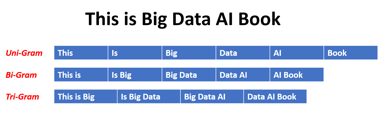
In an N-gram model, the probability of a word is estimated based on its occurrence in the training data relative to its preceding N-1 words. For example, in a trigram model (N=3), the probability of a word is determined by the two words that immediately precede it. This approach assumes that the probability of a word depends only on a fixed number of preceding words and does not consider long-range dependencies.
Here are some examples of n-grams:
Here are the advantages and disadvantages of N-gram language models:
Advantages:
Disadvantages:
Here's an example of using n-grams in Torchtext:
import torchtext
from torchtext.data import get_tokenizer
from torchtext.data.utils import ngrams_iterator

tokenizer = get_tokenizer("basic_english")
# Create a tokenizer object using the "basic_english" tokenizer provided by torchtext
# This tokenizer splits the input text into a list of tokens

tokens = tokenizer("I love to code in Python")
# The result is a list of tokens, where each token represents a word or a punctuation mark

print(list(ngrams_iterator(tokens, 3)))

['i', 'love', 'to', 'code', 'in', 'python', 'i love', 'love to', 'to code', 'code in', 'in python', 'i love to', 'love to code', 'to code in', 'code in python']Note:
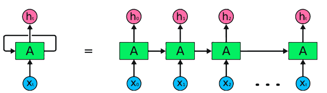
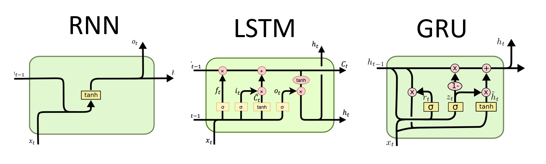
RNNs are the fundamental type of neural network for sequential data processing. They have recurrent connections that allow information to be passed from one step to the next, enabling them to capture dependencies across time. However, traditional RNNs suffer from the vanishing/exploding gradient problem and struggle with long-term dependencies.
Advantages of RNNs:
Disadvantages of RNNs:
PyTorch code snippet for defining a basic RNN in PyTorch:
import torch
import torch.nn as nn

rnn = nn.RNN(input_size=10, hidden_size=20, num_layers=2)
# input_size  – The number of expected features in the input x
# hidden_size – The number of features in the hidden state h
# num_layers  – Number of recurrent layers. E.g., setting num_layers=2 would mean stacking two RNNs together

# Create a randomly initialized input tensor
input = torch.randn(5, 3, 10)  # (sequence length=5, batch size=3, input size=10)

# Create a randomly initialized hidden state tensor
h0 = torch.randn(2, 3, 20)  # (num_layers=2, batch size=3, hidden size=20)

# Apply the RNN module to the input tensor and initial hidden state tensor
output, hn = rnn(input, h0)

print(output.shape)  # torch.Size([5, 3, 20])
# (sequence length=5, batch size=3, hidden size=20)


print(hn.shape)  # torch.Size([2, 3, 20])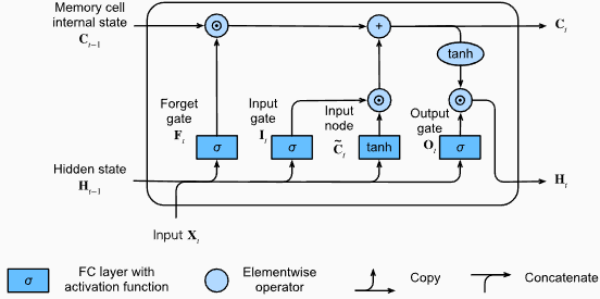
# (num_layers=2, batch size=3, hidden size=20)Advantages of LSTMs:
Disadvantages of LSTMs:
PyTorch code snippet for defining a basic LSTM in PyTorch:
import torch
import torch.nn as nn

input_size = 100
hidden_size = 64
num_layers = 2
batch_size = 1
seq_length = 10

lstm = nn.LSTM(input_size, hidden_size, num_layers)
input_data = torch.randn(seq_length, batch_size, input_size)
h0 = torch.zeros(num_layers, batch_size, hidden_size)
c0 = torch.zeros(num_layers, batch_size, hidden_size)

output, (hn, cn) = lstm(input_data, (h0, c0))
The output shape of the LSTM layer will also be [seq_length, batch_size, hidden_size]. This means that for each input in the sequence, there will be a corresponding output hidden state. In the provided example, the output shape is torch.Size([10, 1, 64]), indicating that the LSTM was applied to a sequence of length 10, with a batch size of 1, and a hidden state size of 64.
Now, let's discuss the hn (hidden state) tensor. Its shape is torch.Size([2, 1, 64]). The first dimension, 2, represents the number of layers in the LSTM. In this case, the num_layers argument was set to 2, so there are 2 layers in the LSTM model. The second dimension, 1, corresponds to the batch size, which is 1 in the given example. Finally, the last dimension, 64, represents the size of the hidden state.
Therefore, the hn tensor contains the final hidden state for each layer of the LSTM after processing the entire input sequence, following the LSTM's ability to retain long-term dependencies and mitigate the vanishing gradient problem.
For more information, please refer to the Long Short-Term Memory (LSTM) chapter in the "Dive into Deep Learning" documentation.
Advantages of GRUs:
Disadvantages of GRUs:
Overall, LSTM and GRU models overcome some of the limitations of traditional RNNs, particularly in capturing long-term dependencies. LSTMs excel in preserving contextual information, while GRUs offer a more computationally efficient alternative. The choice between LSTM and GRU depends on the specific requirements of the task and the available computational resources.
import torch
import torch.nn as nn

input_size = 100
hidden_size = 64
num_layers = 2
batch_size = 1
seq_length = 10

gru = nn.GRU(input_size, hidden_size, num_layers)
input_data = torch.randn(seq_length, batch_size, input_size)
h0 = torch.zeros(num_layers, batch_size, hidden_size)

output, hn = gru(input_data, h0)
The output shape of the GRU layer will also be [seq_length, batch_size, hidden_size]. This means that for each input in the sequence, there will be a corresponding output hidden state. In the provided example, the output shape is torch.Size([10, 1, 64]), indicating that the GRU was applied to a sequence of length 10, with a batch size of 1, and a hidden state size of 64.
Now, let's discuss the hn (hidden state) tensor. Its shape is torch.Size([2, 1, 64]). The first dimension, 2, represents the number of layers in the GRU. In this case, the num_layers argument was set to 2, so there are 2 layers in the GRU model. The second dimension, 1, corresponds to the batch size, which is 1 in the given example. Finally, the last dimension, 64, represents the size of the hidden state.
Therefore, the hn tensor contains the final hidden state for each layer of the GRU after processing the entire input sequence, following the GRU's ability to capture and retain information over long sequences while mitigating the vanishing gradient problem.
For more information, please refer to the Gated Recurrent Units (GRU) chapter in the "Dive into Deep Learning" documentation.
Advantages:
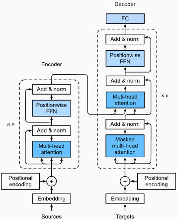
Capturing Long-Range Dependencies: Transformers excel at capturing long-range dependencies in sequences by using self-attention mechanisms. This allows them to consider all positions in the input sequence when making predictions, enabling better understanding of context and improving the quality of generated text.
Parallel Processing: Unlike recurrent models, transformers can process the input sequence in parallel, making them highly efficient and reducing training and inference times. This parallelization is possible due to the absence of sequential dependencies in the architecture.
Scalability: Transformers are highly scalable and can handle large input sequences effectively. They can process sequences of arbitrary lengths without the need for truncation or padding, which is particularly advantageous for tasks involving long documents or sentences.
Contextual Understanding: Transformers can capture rich contextual information by attending to relevant parts of the input sequence. This allows them to understand complex linguistic structures, semantic relationships, and dependencies between words, resulting in more coherent and contextually appropriate language generation.
Disadvantages of Transformer Models:
High Computational Requirements: Transformers typically require significant computational resources compared to simpler models like n-grams or traditional RNNs. Training large transformer models with extensive datasets can be computationally expensive and time-consuming.
Lack of Sequential Modeling: While transformers excel at capturing global dependencies, they may not be as effective at modeling strictly sequential data. In cases where the order of the input sequence is crucial, such as in tasks involving time-series data, traditional RNNs or convolutional neural networks (CNNs) may be more suitable.
Attention Mechanism Complexity: The self-attention mechanism in transformers introduces additional complexity to the model architecture. Understanding and implementing attention mechanisms correctly can be challenging, and tuning hyperparameters related to attention can be non-trivial.
Data Requirements: Transformers often require large amounts of training data to achieve optimal performance. Pretraining on large-scale corpora, such as in the case of pretrained transformer models like GPT and BERT, is common to leverage the power of transformers effectively.
For more information, please refer to the The Transformer Architecture chapter in the "Dive into Deep Learning" documentation.
Despite these limitations, transformer models have revolutionized the field of natural language processing and language modeling. Their ability to capture long-range dependencies and contextual understanding has significantly advanced the state of the art in various language-related tasks, making them a prominent choice for many applications.
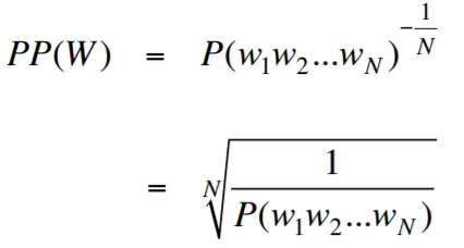
Perplexity, in the context of language modeling, is a measure that quantifies how well a language model predicts a given test set, with lower perplexity indicating better predictive performance. In simpler terms, perplexity is calculated by taking the inverse probability of the test set and then normalizing it by the number of words.
The lower the perplexity value, the better the language model is at predicting the test set. Minimizing perplexity is the same as maximizing probability
The formula for perplexity as the inverse probability of the test set, normalized by the number of words, is as follows:
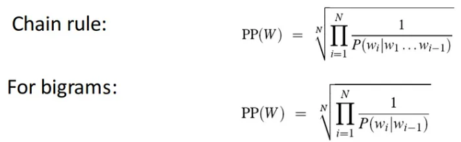
Perplexity can be interpreted as a measure of the branching factor in a language model. The branching factor represents the average number of possible next words or tokens given a particular context or sequence of words.
The Branching factor of a language is the number of possible next words that can follow any word. We can think of perplexity as the weighted average branching factor of a language.
The Language Modeling with Embedding Layer and LSTM code is a powerful tool for building and training language models. This code implementation combines two fundamental components in natural language processing: an embedding layer and a long short-term memory (LSTM) network.
The embedding layer is responsible for converting text data into distributed representations, also known as word embeddings. These embeddings capture semantic and syntactic properties of words, allowing the model to understand the meaning and context of the input text. The embedding layer maps each word in the input sequence to a high-dimensional vector, which serves as the input for subsequent layers in the model.
The LSTM layer in the code implementation processes the word embeddings generated by the embedding layer, capturing the sequence information and learning the underlying patterns and structures in the text.
By combining the embedding layer and LSTM network, the code enables the construction of a language model that can generate coherent and contextually appropriate text. Language models built using this approach can be trained on large textual datasets and are capable of generating realistic and meaningful sentences, making them valuable tools for various natural language processing tasks such as text generation, machine translation, and sentiment analysis.
This code implementation provides a simple, clear, and concise foundation for building language models based on the embedding layer and LSTM architecture. It serves as a starting point for researchers, developers, and enthusiasts who are interested in exploring and experimenting with state-of-the-art language modeling techniques.
Through this code, you can gain a deeper understanding of how embedding layers and LSTMs work together to capture the complex patterns and dependencies within text data. With this knowledge, you can further extend the code and explore advanced techniques, such as incorporating attention mechanisms or transformer architectures, to enhance the performance and capabilities of your language models.
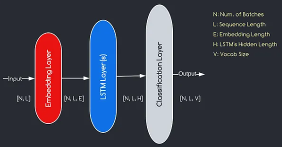
The model we will construct corresponds to the diagram provided above, illustrating the three key components: an embedding layer, LSTM layers, and a classification layer. While the objectives of the LSTM and classification layers are already familiar to us, let's delve into the significance of the embedding layer.
The embedding layer plays a crucial role in the model by transforming each word, represented as an index, into a vector of E dimensions. This vector representation allows subsequent layers to learn and extract meaningful information from the input. It is worth noting that using indices or one-hot vectors to represent words can be inadequate as they assume no relationships between different words.
The mapping process carried out by the embedding layer is a learned procedure that takes place during training. Through this training phase, the model gains the ability to associate words with specific vectors in a way that captures semantic and syntactic relationships, thereby enhancing the model's understanding of the underlying language structure.
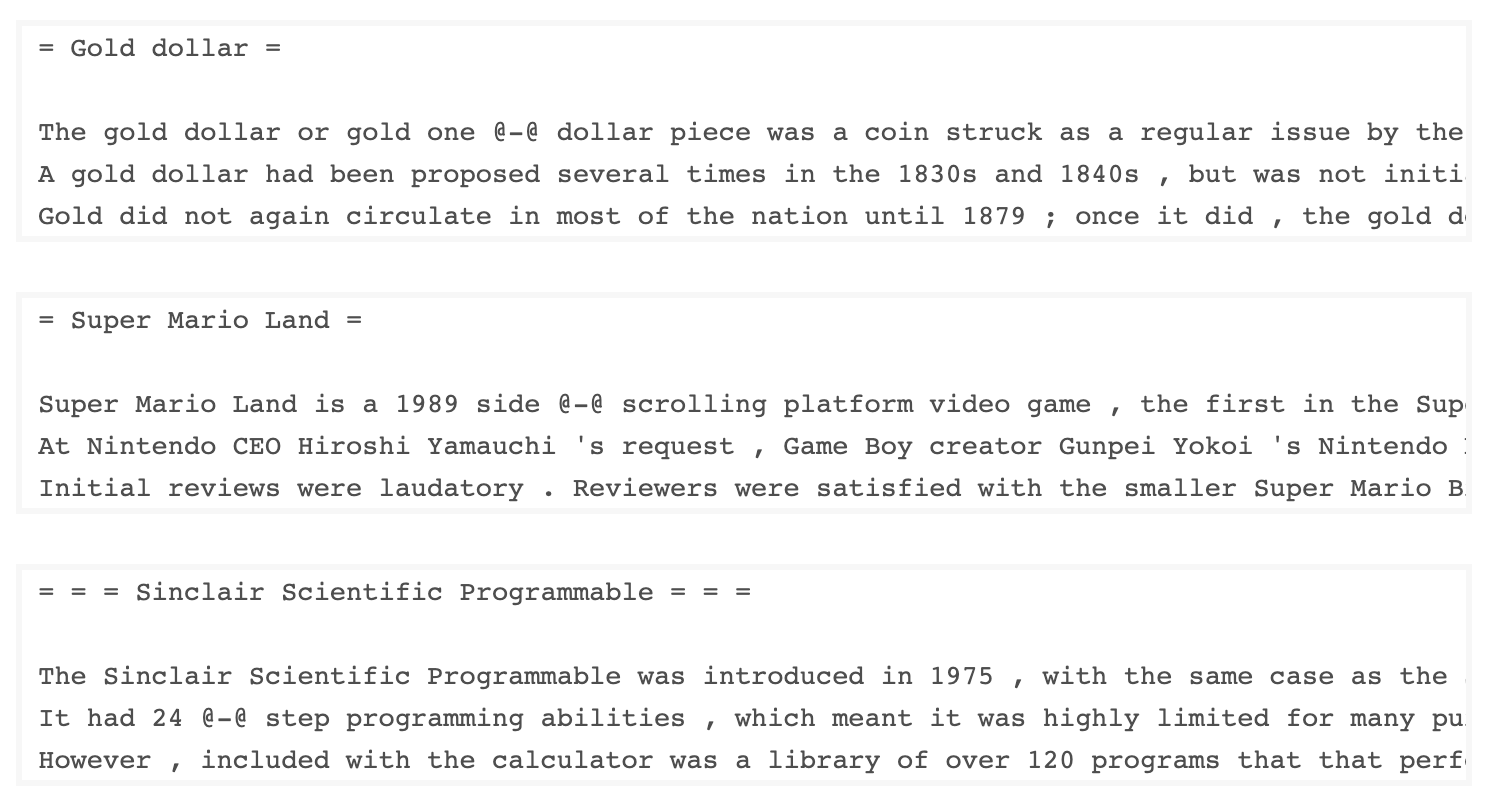
The WkiText-103 dataset, developed by Salesforce, contains over 100 million tokens extracted from the set of verified Good and Featured articles on Wikipedia. It has 267,340 unique tokens that appear at least 3 times in the dataset. Since it has full-length Wikipedia articles, the dataset is well-suited for tasks that can benefit of long term dependencies, such as language modeling.
The WikiText-2 dataset is a small version of the WikiText-103 dataset as it contains only 2 million tokens. This small dataset is suitable for testing your language model.
This repository contains code for performing exploratory data analysis on the UTK dataset, which consists of images categorized by age, gender, and ethnicity.
To download a dataset using Torchtext, you can use the torchtext.datasets module.
Here's an example of how to download the Wikitext-2 dataset using Torchtext:
import torchtext
from torchtext.datasets import WikiText2
data_path = "data"
train_iter, valid_iter, test_iter = WikiText2(root=data_path)
Initially, I tried to use the provided code to load the WikiText-2 dataset, but encountered an issue with the URL (https://s3.amazonaws.com/research.metamind.io/wikitext/wikitext-2-v1.zip) not working for me. To overcome this, I decided to leverage the torchtext library and create a custom implementation of the dataset loader.
Since the original URL was not working, I downloaded the train, validation, and test datasets from a GitHub repository and placed them in the 'data/datasets/WikiText2' directory.
Here's a breakdown of the code:
import os
from typing import Union, Tuple

from torchdata.datapipes.iter import FileOpener, IterableWrapper
from torchtext.data.datasets_utils import _wrap_split_argument, _create_dataset_directory

DATA_DIR = "data"

NUM_LINES = {
    "train": 36718,
    "valid": 3760,
    "test": 4358,
}

DATASET_NAME = "WikiText2"

_EXTRACTED_FILES = {
    "train": "wiki.train.tokens",
    "test": "wiki.test.tokens",
    "valid": "wiki.valid.tokens",
}


def _filepath_fn(root, split):
    return os.path.join(root, _EXTRACTED_FILES[split])


@_create_dataset_directory(dataset_name=DATASET_NAME)
@_wrap_split_argument(("train", "valid", "test"))

def WikiText2(root: str, split: Union[Tuple[str], str]):
    url_dp = IterableWrapper([_filepath_fn(DATA_DIR, split)])
    data_dp = FileOpener(url_dp, encoding="utf-8").readlines(strip_newline=False, return_path=False).shuffle().set_shuffle(False).sharding_filter()
return data_dpTo use the WikiText-2 dataset loader, simply import the WikiText2 function and call it with the desired data split:
train_data = WikiText2(root="data/datasets/WikiText2", split="train")
valid_data = WikiText2(root="data/datasets/WikiText2", split="valid")
test_data = WikiText2(root="data/datasets/WikiText2", split="test")This implementation is inspired by the official torchtext dataset loaders, and leverages the torchdata and torchtext libraries to provide a seamless and efficient data loading experience.
Building a vocabulary is a crucial step in many natural language processing tasks, as it allows you to represent words as unique identifiers that can be used in machine learning models. This Markdown document demonstrates how to build a vocabulary from a set of training data and save it for future use.
Here's a function that encapsulates the process of building and saving a vocabulary:
import torch
from torchtext.data.utils import get_tokenizer
from torchtext.vocab import build_vocab_from_iterator

def build_and_save_vocabulary(train_iter, vocab_path='vocab.pt', min_freq=4):
    """
    Build a vocabulary from the training data iterator and save it to a file.

    Args:
        train_iter (iterator): An iterator over the training data.
        vocab_path (str, optional): The path to save the vocabulary file. Defaults to 'vocab.pt'.
        min_freq (int, optional): The minimum frequency of a word to be included in the vocabulary. Defaults to 4.

    Returns:
        torchtext.vocab.Vocab: The built vocabulary.
    """
    # Get the tokenizer
    tokenizer = get_tokenizer("basic_english")

    # Build the vocabulary
    vocab = build_vocab_from_iterator(map(tokenizer, train_iter), specials=['<unk>'], min_freq=min_freq)

    # Set the default index to the unknown token
    vocab.set_default_index(vocab['<unk>'])

    # Save the vocabulary
    torch.save(vocab, vocab_path)

    return vocab
Here's how you can use this function:
# Assuming you have a training data iterator named `train_iter`
vocab = build_and_save_vocabulary(train_iter, vocab_path='my_vocab.pt')

# You can now use the vocabulary
print(len(vocab))  # 23652
print(vocab(['ebi', 'AI'.lower(), 'qwerty'])) # [0, 1973, 0]build_and_save_vocabulary function takes three arguments: train_iter (an iterator over the training data), vocab_path (the path to save the vocabulary file, with a default of 'vocab.pt'), and min_freq (the minimum frequency of a word to be included in the vocabulary, with a default of 4).basic_english tokenizer, which performs basic tokenization on English text.build_vocab_from_iterator function, passing the training data iterator (after tokenization) and specifying the '<unk>' special token and the minimum frequency threshold.'<unk>' token, which means that any word not found in the vocabulary will be mapped to the unknown token.To use this function, you need to have a training data iterator named train_iter. Then, you can call the build_and_save_vocabulary function, passing the train_iter and specifying the desired vocabulary file path and minimum frequency threshold.
The function will build the vocabulary, save it to the specified file, and return the Vocab object, which you can then use in your downstream tasks.
This code provides a way to analyze the mean sentence length in the Wikitext-2 dataset. Here's a breakdown of the code:
import matplotlib.pyplot as plt

def compute_mean_sentence_length(data_iter):
    """
    Computes the mean sentence length for the given data iterator.

    Args:
        data_iter (iterable): An iterable of text data, where each element is a string representing a line of text.

    Returns:
        float: The mean sentence length.
    """
    total_sentence_count = 0
    total_sentence_length = 0

    for line in data_iter:
        sentences = line.split('.')  # Split the line into individual sentences

        for sentence in sentences:
            tokens = sentence.strip().split()  # Tokenize the sentence
            sentence_length = len(tokens)

            if sentence_length > 0:
                total_sentence_count += 1
                total_sentence_length += sentence_length

    mean_sentence_length = total_sentence_length / total_sentence_count
    return mean_sentence_length

# Compute mean sentence length for each dataset
train_mean = compute_mean_sentence_length(train_iter)
valid_mean = compute_mean_sentence_length(valid_iter)
test_mean  = compute_mean_sentence_length(test_iter)

# Plot the results
datasets = ['Train', 'Valid', 'Test']
means = [train_mean, valid_mean, test_mean]

plt.figure(figsize=(6, 4))
plt.bar(datasets, means)
plt.xlabel('Dataset')
plt.ylabel('Mean Sentence Length')
plt.title('Mean Sentence Length in Wikitext-2')
plt.grid(True)
plt.show()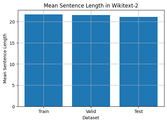
from collections import Counter

# Compute word frequencies in the training dataset
freqs = Counter()
for tokens in map(tokenizer, train_iter):
    freqs.update(tokens)

# Find the 10 least common words
least_common_words = freqs.most_common()[:-11:-1]
print("Least Common Words:")
for word, count in least_common_words:
    print(f"{word}: {count}")

# Find the 10 most common words
most_common_words = freqs.most_common(10)
print("nMost Common Words:")
for word, count in most_common_words:
print(f"{word}: {count}")from collections import Counter
# Compute word frequencies in the training dataset
freqs = Counter()
for tokens in map(tokenizer, train_iter):
freqs.update(tokens)
# Count the number of words that repeat 3, 4, and 5 times
count_3 = count_4 = count_5 = 0
for word, freq in freqs.items():
if freq == 3:
count_3 += 1
elif freq == 4:
count_4 += 1
elif freq == 5:
count_5 += 1
print(f"Number of words that appear 3 times: {count_3}") # 5130
print(f"Number of words that appear 4 times: {count_4}") # 3243
print(f"Number of words that appear 5 times: {count_5}") # 2261from collections import Counter
import matplotlib.pyplot as plt
# Compute the word lengths in the training dataset
word_lengths = []
for tokens in map(tokenizer, train_iter):
word_lengths.extend(len(word) for word in tokens)
# Create a frequency distribution of word lengths
word_length_counts = Counter(word_lengths)
# Plot the word length distribution
plt.figure(figsize=(10, 6))
plt.bar(word_length_counts.keys(), word_length_counts.values())
plt.xlabel("Word Length")
plt.ylabel("Frequency")
plt.title("Word Length Distribution in Wikitext-2 Dataset")
plt.show()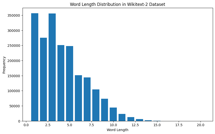
import spacy
import en_core_web_sm

# Load the small English language model from SpaCy
nlp = spacy.load("en_core_web_sm")

# Alternatively, you can use the en_core_web_sm module to load the model
nlp = en_core_web_sm.load()

# Process the given sentence using the loaded language model
doc = nlp("This is a sentence.")

# Print the text and part-of-speech tag for each token in the sentence
print([(w.text, w.pos_) for w in doc])

# [('This', 'PRON'), ('is', 'AUX'), ('a', 'DET'), ('sentence', 'NOUN'), ('.', 'PUNCT')]
For Wikitext-2 dataset:
import spacy

# Load the English language model
nlp = spacy.load("en_core_web_sm")

# Perform POS tagging on the training dataset
pos_tags = []
for tokens in map(tokenizer, train_iter):
    doc = nlp(" ".join(tokens))
    pos_tags.extend([(token.text, token.pos_) for token in doc])

# Count the frequency of each POS tag
pos_tag_counts = Counter(tag for _, tag in pos_tags)

# Print the most common POS tags
print("Most Common Part-of-Speech Tags:")
for tag, count in pos_tag_counts.most_common(10):
    print(f"{tag}: {count}")

# Visualize the POS tag distribution
plt.figure(figsize=(12, 6))
plt.bar(pos_tag_counts.keys(), pos_tag_counts.values())
plt.xticks(rotation=90)
plt.xlabel("Part-of-Speech Tag")
plt.ylabel("Frequency")
plt.title("Part-of-Speech Tag Distribution in Wikitext-2 Dataset")
plt.show()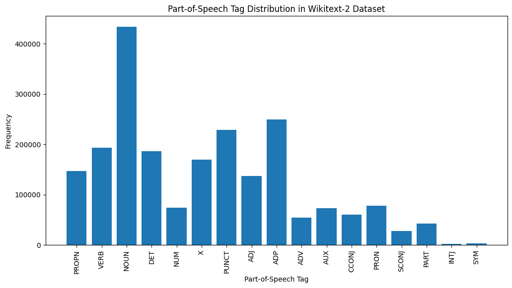
Here's a brief explanation of the most common POS tags in the provided output:
NOUN: Nouns represent people, places, things, or ideas.
ADP: Adpositions, such as prepositions and postpositions, are used to express relationships between words or phrases.
PUNCT: Punctuation marks, which are essential for separating and structuring sentences and text.
VERB: Verbs describe actions, states, or occurrences in the text.
DET: Determiners, such as articles (e.g., "the," "a," "an"), provide additional information about nouns.
X: This tag is often used for foreign words, abbreviations, or other language-specific tokens that don't fit into the standard POS categories.
PROPN: Proper nouns, which represent specific names of people, places, organizations, or other entities.
ADJ: Adjectives modify or describe nouns and pronouns.
PRON: Pronouns substitute for nouns, making the text more concise and less repetitive.
NUM: Numerals, which represent quantities, dates, or other numerical information.
This distribution of POS tags can provide insights into the linguistic characteristics of the text, such as the predominance of nouns, the prevalence of adpositions, or the usage of proper nouns, which can be helpful in tasks like text classification, information extraction, or stylometric analysis.
import spacy
import matplotlib.pyplot as plt

# Load the English language model
nlp = spacy.load("en_core_web_sm")

# Perform NER on the training dataset
named_entities = []
for tokens in map(tokenizer, train_iter):
    doc = nlp(" ".join(tokens))
    named_entities.extend([(ent.text, ent.label_) for ent in doc.ents])

# Count the frequency of each named entity type
ner_counts = Counter(label for _, label in named_entities)

# Print the most common named entity types
print("Most Common Named Entity Types:")
for label, count in ner_counts.most_common(10):
    print(f"{label}: {count}")

# Visualize the named entity distribution
plt.figure(figsize=(12, 6))
plt.bar(ner_counts.keys(), ner_counts.values())
plt.xticks(rotation=90)
plt.xlabel("Named Entity Type")
plt.ylabel("Frequency")
plt.title("Named Entity Distribution in Wikitext-2 Dataset")
plt.show()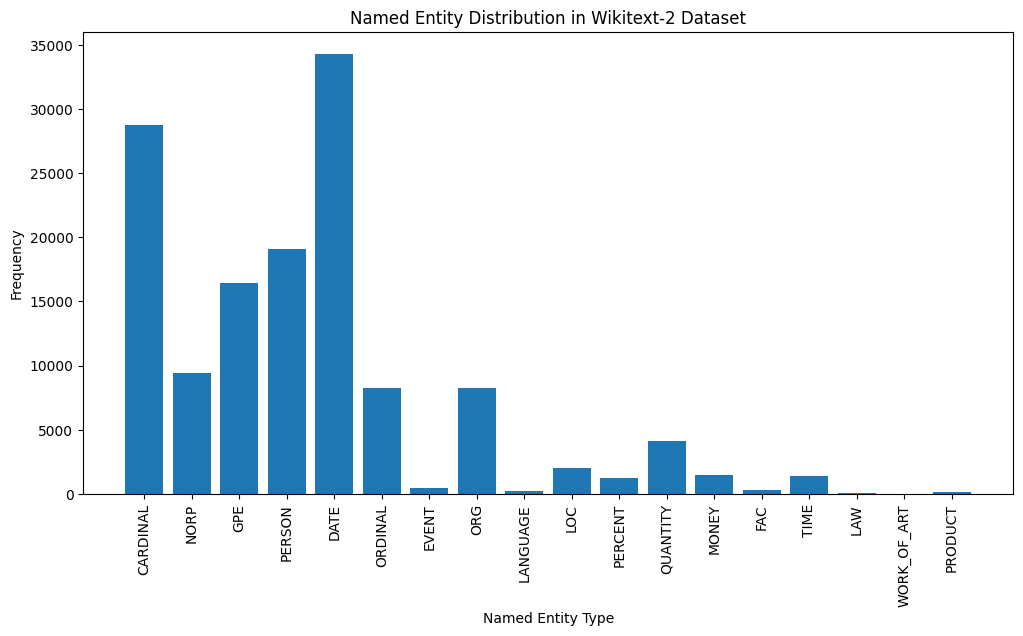
Here's a brief explanation of the most common named entity types in the output:
DATE: Represents specific dates, time periods, or temporal expressions, such as "June 15, 2024" or "last year".
CARDINAL: Includes numerical values, such as quantities, ages, or measurements.
PERSON: Identifies the names of individual people.
GPE (Geopolitical Entity): This entity type represents named geographical locations, such as countries, cities, or states.
NORP (Nationalities, Religious, or Political Groups): This entity type includes named groups or affiliations based on nationality, religion, or political ideology.
ORDINAL: Represents ordinal numbers, such as "first," "second," or "3rd".
ORG (Organization): The names of companies, institutions, or other organized groups.
QUANTITY: Includes non-numeric quantities, such as "a few" or "several".
LOC (Location): Represents named geographical locations, such as continents, regions, or landforms.
MONEY: Identifies monetary values, such as dollar amounts or currency names.
This distribution of named entity types can provide valuable insights into the content and focus of the text. For example, the prominence of DATE and CARDINAL entities may suggest a text that deals with numerical or temporal information, while the prevalence of PERSON, ORG, and GPE entities could indicate a text that discusses people, organizations, and geographical locations.
Understanding the named entity distribution can be useful in a variety of applications, such as information extraction, question answering, and text summarization, where identifying and categorizing key named entities is crucial for understanding the context and content of the text.
from wordcloud import WordCloud
import matplotlib.pyplot as plt

# Load the training dataset
with open("data/wiki.train.tokens", "r") as f:
    train_text = f.read().split()

# Create a string from the entire training dataset
text = " ".join(train_text)

# Generate the word cloud
wordcloud = WordCloud(width=800, height=400, background_color='white').generate(text)

# Plot the word cloud
plt.figure(figsize=(12, 8))
plt.imshow(wordcloud, interpolation='bilinear')
plt.axis('off')
plt.title('Word Cloud for Wikitext-2 Training Dataset')
plt.show()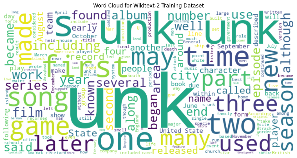
from sentence_transformers import SentenceTransformer
from sklearn.cluster import KMeans
from collections import defaultdict
from wordcloud import WordCloud
import matplotlib.pyplot as plt

# Load the BERT-based sentence transformer model
model = SentenceTransformer('bert-base-nli-mean-tokens')

# Load the training dataset
with open("data/wiki.valid.tokens", "r") as f:
    train_text = f.read().split()

# Compute the BERT embeddings for each unique word in the dataset
unique_words = set(train_text)
word_embeddings = model.encode(list(unique_words))

# Cluster the words using K-Means
num_clusters = 5
kmeans = KMeans(n_clusters=num_clusters, random_state=42)
clusters = kmeans.fit_predict(word_embeddings)

# Group the words by cluster
word_clusters = defaultdict(list)
for i, word in enumerate(unique_words):
    word_clusters[clusters[i]].append(word)

# Create a word cloud for each cluster
fig, axes = plt.subplots(1, 5, figsize=(14, 12))
axes = axes.flatten()

for cluster_id, cluster_words in word_clusters.items():
    word_cloud = WordCloud(width=400, height=200, background_color='white').generate(' '.join(cluster_words))
    axes[cluster_id].imshow(word_cloud, interpolation='bilinear')
    axes[cluster_id].set_title(f"Cluster {cluster_id}")
    axes[cluster_id].axis('off')

plt.subplots_adjust(wspace=0.4, hspace=0.6)

plt.tight_layout()
plt.show()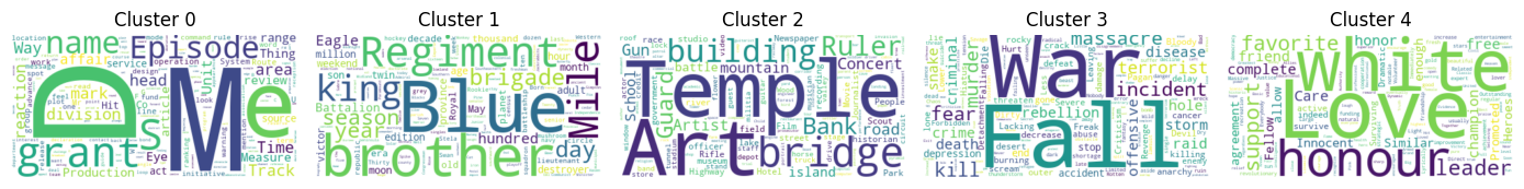
The two data formats, N x B x L and M x L, are commonly used in language modeling tasks, particularly in the context of neural network-based models.
N x B x L format:
N represents the number of batches. In this case, the dataset is divided into N smaller batches, which is a common practice to improve the efficiency and stability of the training process.B is the batch size, which represents the number of samples (e.g., sentences, paragraphs, or documents) within each batch.L is the length of a sample within each batch, which typically corresponds to the number of tokens (words) in a sample.M x L format:
N x B x L format.M is equal to N x B, which represents the total number of samples (e.g., sentences, paragraphs, or documents) in the dataset.L is the length of each sample, which corresponds to the number of tokens (words) in the sample.The choice between these two formats depends on the specific requirements of your language modeling task and the capabilities of the neural network architecture you're working with. If you're training a neural network-based language model, the N x B x L format is typically preferred, as it allows for efficient batch-based training and can lead to faster convergence and better performance. However, if your task doesn't involve neural networks or if the dataset is relatively small, the M x L format may be more suitable.
def prepare_language_model_data(raw_text_iterator, sequence_length):
    """
    Prepare PyTorch tensors for a language model.

    Args:
        raw_text_iterator (iterable): An iterator of raw text data.
        sequence_length (int): The length of the input and target sequences.

    Returns:
        tuple: A tuple containing two PyTorch tensors:
            - inputs (torch.Tensor): A tensor of input sequences.
            - targets (torch.Tensor): A tensor of target sequences.
    """
    # Convert the raw text iterator into a single PyTorch tensor
    data = torch.cat([torch.LongTensor(vocab(tokenizer(line))) for line in raw_text_iterator])

    # Calculate the number of complete sequences that can be formed
    num_sequences = len(data) // sequence_length

    # Calculate the remainder of the data length divided by the sequence length
    remainder = len(data) % sequence_length

    # If the remainder is 0, add a single <unk> token to the end of the data tensor
    if remainder == 0:
        unk_tokens = torch.LongTensor([vocab['<unk>']])
        data = torch.cat([data, unk_tokens])

    # Extract the input and target sequences from the data tensor
    inputs = data[:num_sequences*sequence_length].reshape(-1, sequence_length)
    targets = data[1:num_sequences*sequence_length+1].reshape(-1, sequence_length)

    print(len(inputs), len(targets))
return inputs, targetssequence_length = 30
X_train, y_train = prepare_language_model_data(train_iter, sequence_length)
X_valid, y_valid = prepare_language_model_data(valid_iter, sequence_length)
X_test, y_test = prepare_language_model_data(test_iter, sequence_length)
X_train.shape, y_train.shape, X_valid.shape, y_valid.shape, X_test.shape, y_test.shape
(torch.Size([68333, 30]),
torch.Size([68333, 30]),
torch.Size([7147, 30]),
torch.Size([7147, 30]),
torch.Size([8061, 30]),
torch.Size([8061, 30]))This code defines a PyTorch Dataset class for working with language model data. The LanguageModelDataset class takes in input and target tensors and provides the necessary methods for accessing the data.
class LanguageModelDataset(Dataset):
    def __init__(self, inputs, targets):
        self.inputs = inputs
        self.targets = targets

    def __len__(self):
        return self.inputs.shape[0]

    def __getitem__(self, idx):
return self.inputs[idx], self.targets[idx]The LanguageModelDataset class can be used as follows:
# Create the datasets
train_set = LanguageModelDataset(X_train, y_train)
valid_set = LanguageModelDataset(X_valid, y_valid)
test_set  = LanguageModelDataset(X_test, y_test)

# Create data loaders (optional)
train_loader = DataLoader(train_set, batch_size=32, shuffle=True)
valid_loader = DataLoader(valid_set, batch_size=32)
test_loader  = DataLoader(test_set, batch_size=32)

# Access the data
x_batch, y_batch = next(iter(train_loader))
print(f"Input batch shape: {x_batch.shape}")  # Input batch shape: torch.Size([32, 30])
print(f"Target batch shape: {y_batch.shape}") # Target batch shape: torch.Size([32, 30])The code defines a custom PyTorch language model that allows you to use different types of word embeddings, including randomly initialized embeddings, pre-trained GloVe embeddings, pre-trained FastText embeddings, by simply specifying the embedding_type argument when creating the model instance.
import torch.nn as nn
from torchtext.vocab import GloVe, FastText


class LanguageModel(nn.Module):
    def __init__(self, vocab_size, embedding_dim,
                 hidden_dim, num_layers, dropout_embd=0.5,
                 dropout_rnn=0.5, embedding_type='random'):

        super().__init__()
        self.num_layers = num_layers
        self.hidden_dim = hidden_dim
        self.embedding_dim = embedding_dim
        self.embedding_type = embedding_type

        if embedding_type == 'random':
            self.embedding = nn.Embedding(vocab_size, embedding_dim)
            self.embedding.weight.data.uniform_(-0.1, 0.1)

        elif embedding_type == 'glove':
            self.glove = GloVe(name='6B', dim=embedding_dim)
            self.embedding = nn.Embedding(vocab_size, embedding_dim)
            self.embedding.weight.data.copy_(self.glove.vectors)
            self.embedding.weight.requires_grad = False

        elif embedding_type == 'fasttext':
            self.glove = FastText(language='en')
            self.embedding = nn.Embedding(vocab_size, embedding_dim)
            self.embedding.weight.data.copy_(self.fasttext.vectors)
            self.embedding.weight.requires_grad = False

        else:
            raise ValueError("Invalid embedding_type. Choose from 'random', 'glove', 'fasttext'.")

        self.dropout = nn.Dropout(p=dropout_embd)
        self.lstm = nn.LSTM(embedding_dim, hidden_dim, num_layers=num_layers,
                           dropout=dropout_rnn, batch_first=True)
        self.fc = nn.Linear(hidden_dim, vocab_size)

    def forward(self, src):
        embedding = self.dropout(self.embedding(src))
        output, hidden = self.lstm(embedding)
        prediction = self.fc(output)
return predictionmodel = LanguageModel(vocab_size=len(vocab),
embedding_dim=300,
hidden_dim=512,
num_layers=2,
dropout_embd=0.65,
dropout_rnn=0.5,
embedding_type='glove')def num_trainable_params(model):
nums = sum(p.numel() for p in model.parameters() if p.requires_grad) / 1e6
return nums
# Calculate the number of trainable parameters in the embedding, LSTM, and fully connected layers of the LanguageModel instance 'model'
num_trainable_params(model.embedding) # (7.0956)
num_trainable_params(model.lstm) # (3.76832)
num_trainable_params(model.fc) # (12.133476)

