Torch Linguist
1.0.0
该项目是使用Pytorch构建语言模型的分步指南。它旨在对开发语言模型及其应用程序所涉及的过程进行全面的了解。
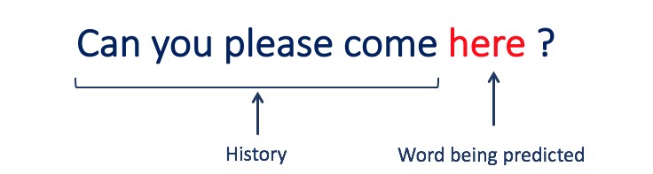
语言建模或LM是使用各种统计和概率技术来确定句子中出现的单词序列的概率。语言模型分析文本数据的机构,为其单词预测提供基础。
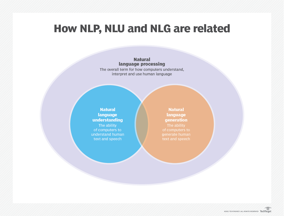
语言建模用于人工智能(AI),自然语言处理(NLP),自然语言理解(NLU)和自然语言生成(NLG)系统,尤其是执行文本生成,机器翻译和问题答案的系统。
大型语言模型(LLMS)还使用语言建模。这些是高级语言模型,例如OpenAI的GPT-3和Google的Palm 2,它们处理数十亿个培训数据参数并生成文本输出。
通常使用跨凝结和困惑等指标来评估语言模型的有效性,这些指标衡量了模型准确预测下一个单词的能力(我将在步骤2中介绍它们)。几个数据集,例如Wikitext-2,Wikitext-103,十亿个单词,Text8和C4等,通常用于评估语言模型。注意:在此项目中,我使用Wikitext-2。
LM的研究在文献中受到了广泛的关注,可以将其分为四个主要的发展阶段:
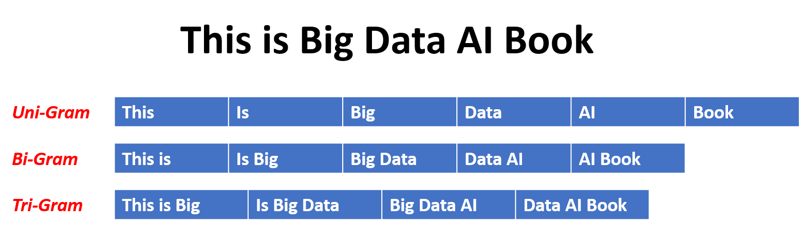
SLM是基于1990年代升起的统计学习方法而开发的。基本思想是基于马尔可夫假设(例如,根据最新上下文预测下一个单词)构建单词预测模型。具有固定上下文长度n的SLM也称为N-Gram语言模型,例如,Bigram和Trigram语言模型。 SLM已被广泛应用于提高信息检索(IR)和自然语言处理(NLP)的任务性能。但是,他们经常受到维度的诅咒:
由于需要估算指数次数的过渡概率,因此很难准确估计高阶语言模型。因此,已经引入了专门设计的平滑策略,例如退缩估计和良好的估算,以减轻数据稀疏问题。
NLMS通过神经网络,例如,多层感知器(MLP)和复发性神经网络(RNN)来表征单词序列的概率。作为非凡的贡献,是分布式表示的概念。分布式表示形式(也称为嵌入式)的想法是,数据点的“含义”或“语义内容”分布在多个维度上。例如,在NLP中,具有相似含义的单词被映射到彼此接近的向量空间中的点。这种亲密关系不是任意的,而是从单词出现的上下文中学到的。这种与上下文相关的学习通常是通过神经网络模型(例如Word2Vec或Glove )来实现的,该模型会处理大量文本以学习这些表示形式。
分布式表示形式的关键优势之一是它们捕获细粒语义关系的能力。例如,在训练有素的单词嵌入空间中,同义词将由近距离的向量表示,甚至可以使用这些向量对应于有意义的语义操作(例如,“ king” - “男人” - “男人” +“女人”的矢量进行算术操作,可能会导致矢量接近“ Queen”)。
分布式表示的应用:
分布式表示形式具有广泛的应用,尤其是在涉及自然语言理解的任务中。它们用于:
单词相似性:测量单词之间的语义相似性。
文本分类:将文档分类为预定义的类。
机器翻译:将文本从一种语言转换为另一种语言。
信息检索:查找有关查询的相关文档。
情感分析:确定文本中表达的情感。
此外,分布式表示不限于文本数据。它们还可以应用于其他类型的数据,例如图像,其中深度学习模型学会将图像表示为捕获视觉特征和语义的高维向量。
因果语言模型(也称为自回归模型)通过以前单词的顺序预测下一个单词来生成文本。这些模型经过训练,以最大程度地利用变压器体系结构等技术来最大程度地提高下一个单词的可能性。在训练过程中,该模型的输入是整个序列,直到给定令牌,该模型的目标是预测下一个令牌。这种类型的模型对于诸如文本生成,完成和摘要等任务很有用。
蒙版语言模型(MLMS)旨在通过预测句子中的蒙版或丢失单词来学习单词的上下文表示。在训练过程中,一部分输入序列被随机掩盖,并训练该模型以预测给定上下文的原始单词。 MLMS使用诸如变形金刚之类的双向体系结构来捕获蒙版单词和句子其余部分之间的依赖关系。这些模型在诸如文本分类,命名实体识别和问题答案之类的任务中表现出色。
训练序列到序列(SEQ2SEQ)模型以将输入序列映射到输出序列。它们由处理输入序列的编码器和生成输出序列的解码器组成。 SEQ2SEQ模型被广泛用于机器翻译,文本摘要和对话系统等任务。可以使用诸如复发神经网络(RNN)或变形金刚等技术进行训练。训练目标是最大化给定输入的正确输出顺序的可能性。
重要的是要注意,这些培训方法不是相互排斥的,研究人员经常将它们结合起来或采用变化来实现特定目标。例如,诸如T5之类的模型结合了自回归和掩盖的语言模型培训目标,以学习各种任务。
每种培训方法都有其自己的优势和劣势,并且模型的选择取决于特定的任务要求和可用培训数据。
有关更多信息,请参阅“ Medium.com”网站上的语言模型培训方法指南。
语言建模涉及构建可以生成或预测单词或字符序列的模型。以下是一些通常用于语言建模的不同类型的模型:
在n-gram模型中,单词的概率是根据训练数据相对于其先前的n-1单词在训练数据中的出现而估计的。例如,在Trigram模型(n = 3)中,单词的概率由紧接其之前的两个单词确定。这种方法假定单词的概率仅取决于上一个固定数量的单词,并且不考虑长期依赖性。
以下是n-grams的一些示例:
这是N-Gram语言模型的优点和缺点:
优点:
缺点:
这是在torchtext中使用n-grams的示例:
 import torchtext
from torchtext . data import get_tokenizer
from torchtext . data . utils import ngrams_iterator

tokenizer = get_tokenizer ( "basic_english" )
# Create a tokenizer object using the "basic_english" tokenizer provided by torchtext
# This tokenizer splits the input text into a list of tokens

tokens = tokenizer ( "I love to code in Python" )
# The result is a list of tokens, where each token represents a word or a punctuation mark

print ( list ( ngrams_iterator ( tokens , 3 )))

[ 'i' , 'love' , 'to' , 'code' , 'in' , 'python' , 'i love' , 'love to' , 'to code' , 'code in' , 'in python' , 'i love to' , 'love to code' , 'to code in' , 'code in python' ]笔记:
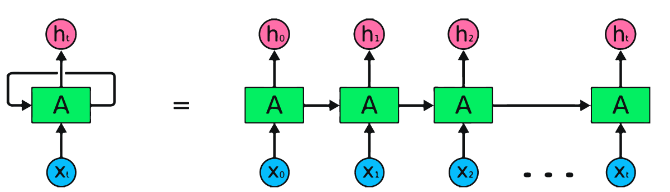
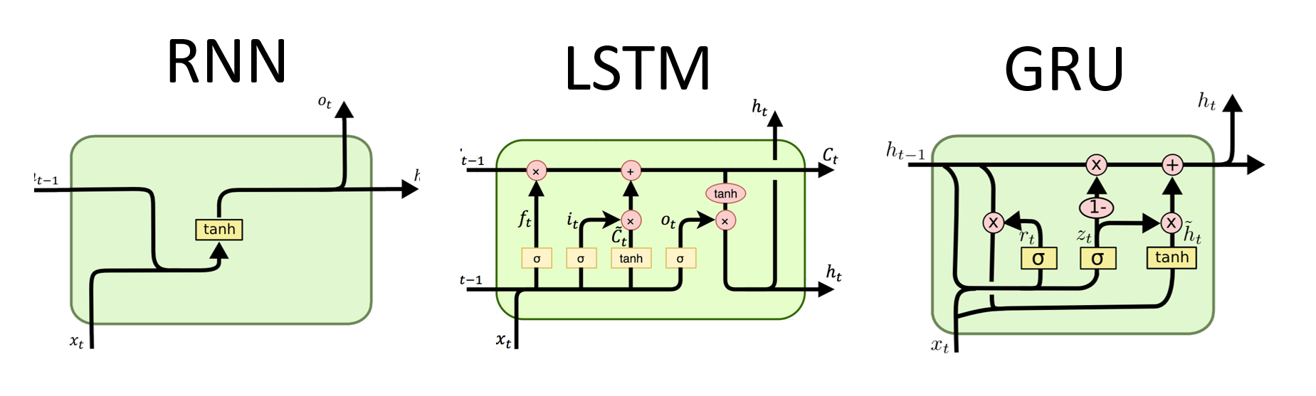
RNN是用于顺序数据处理的神经网络的基本类型。它们具有循环连接,允许信息从一个步骤传递到另一个步骤,从而使他们能够跨时间捕获依赖关系。但是,传统的RNN遭受了消失/爆炸的梯度问题,并在长期依赖方面挣扎。
RNN的优势:
RNN的缺点:
Pytorch代码段用于定义Pytorch中的基本RNN:
 import torch
import torch . nn as nn

rnn = nn . RNN ( input_size = 10 , hidden_size = 20 , num_layers = 2 )
# input_size  – The number of expected features in the input x
# hidden_size – The number of features in the hidden state h
# num_layers  – Number of recurrent layers. E.g., setting num_layers=2 would mean stacking two RNNs together

# Create a randomly initialized input tensor
input = torch . randn ( 5 , 3 , 10 )  # (sequence length=5, batch size=3, input size=10)

# Create a randomly initialized hidden state tensor
h0 = torch . randn ( 2 , 3 , 20 )  # (num_layers=2, batch size=3, hidden size=20)

# Apply the RNN module to the input tensor and initial hidden state tensor
output , hn = rnn ( input , h0 )

print ( output . shape )  # torch.Size([5, 3, 20])
# (sequence length=5, batch size=3, hidden size=20)


print ( hn . shape )  # torch.Size([2, 3, 20])
# (num_layers=2, batch size=3, hidden size=20)LSTMS的优势:
LSTMS的缺点:
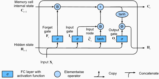
Pytorch代码段用于定义Pytorch中的基本LSTM:
 import torch
import torch . nn as nn

input_size = 100
hidden_size = 64
num_layers = 2
batch_size = 1
seq_length = 10

lstm = nn . LSTM ( input_size , hidden_size , num_layers )
input_data = torch . randn ( seq_length , batch_size , input_size )
h0 = torch . zeros ( num_layers , batch_size , hidden_size )
c0 = torch . zeros ( num_layers , batch_size , hidden_size )

output , ( hn , cn ) = lstm ( input_data , ( h0 , c0 )) LSTM层的输出形状也将是[seq_length, batch_size, hidden_size] 。这意味着,对于序列中的每个输入,将有一个相应的输出隐藏状态。在提供的示例中,输出形状为torch.Size([10, 1, 64]) ,表明LSTM应用于长度10的序列,批量大小为1,隐藏状态大小为64。
现在,让我们讨论hn (隐藏状态)张量。它的形状为torch.Size([2, 1, 64]) 。第一个维度2表示LSTM中的层数。在这种情况下, num_layers参数设置为2,因此LSTM模型中有2层。第二维1,对应于批处理大小,在给定的示例中为1。最后,最后一个维度为64表示隐藏状态的大小。
因此,遵循LSTM保留长期依赖性并减轻消失的梯度问题后, hn张量包含LSTM每一层的最终隐藏状态。
有关更多信息,请参阅“深入深入学习”文档中的长期短期记忆(LSTM)章节。
格鲁斯的优势:
格鲁斯的缺点:
总体而言,LSTM和GRU模型克服了传统RNN的某些局限性,尤其是在捕获长期依赖方面。 LSTMS在保留上下文信息方面表现出色,而GRU提供了更有效的替代方案。 LSTM和GRU之间的选择取决于任务的特定要求和可用的计算资源。
 import torch
import torch . nn as nn

input_size = 100
hidden_size = 64
num_layers = 2
batch_size = 1
seq_length = 10

gru = nn . GRU ( input_size , hidden_size , num_layers )
input_data = torch . randn ( seq_length , batch_size , input_size )
h0 = torch . zeros ( num_layers , batch_size , hidden_size )

output , hn = gru ( input_data , h0 ) GRU层的输出形状也将是[seq_length, batch_size, hidden_size] 。这意味着,对于序列中的每个输入,将有一个相应的输出隐藏状态。在提供的示例中,输出形状为torch.Size([10, 1, 64]) ,表明GRU应用于长度10的序列,批量大小为1,隐藏状态大小为64。
现在,让我们讨论hn (隐藏状态)张量。它的形状为torch.Size([2, 1, 64]) 。第一个维度为2表示GRU中的层数。在这种情况下, num_layers参数设置为2,因此GRU模型中有2层。第二维1,对应于批处理大小,在给定的示例中为1。最后,最后一个维度为64表示隐藏状态的大小。
因此, hn张量在处理整个输入序列后,遵循GRU捕获和保留长序列的信息,同时减轻消失的梯度问题,在处理整个输入序列后,包含GRU每一层的最终隐藏状态。
有关更多信息,请参阅“深入深入学习”文档中的封闭式复发单元(GRU)章节。
优点:
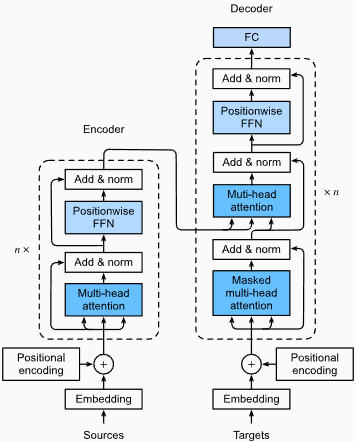
捕获远程依赖性:变形金刚通过使用自我注意的机制在序列中捕获长距离依赖性方面表现出色。这使他们可以在做出预测时考虑输入序列中的所有位置,从而更好地理解上下文并提高生成的文本质量。
并行处理:与复发模型不同,变压器可以并行处理输入序列,从而使其高效且减少训练时间和推理时间。由于体系结构中没有顺序依赖性,因此可以进行这种并行化。
可扩展性:变压器具有高度扩展性,可以有效处理大型输入序列。他们可以处理任意长度的序列而无需截断或填充,这对于涉及长文档或句子的任务尤其有利。
上下文理解:变压器可以通过参与输入序列的相关部分来捕获丰富的上下文信息。这使他们能够理解单词之间复杂的语言结构,语义关系和依赖性,从而导致更连贯和上下文适当的语言产生。
变压器模型的缺点:
较高的计算要求:与N-Grams或传统RNN(N-Grams或传统的RNN)相比,变压器通常需要大量的计算资源。使用大量数据集的培训大型变压器模型在计算上可能是昂贵且耗时的。
缺乏顺序建模:当变压器在捕获全局依赖性方面表现出色时,它们可能在对严格的顺序数据进行建模方面可能不那么有效。如果输入序列的顺序至关重要,例如在涉及时间序列数据的任务中,传统的RNN或卷积神经网络(CNN)可能更合适。
注意机制的复杂性:变形金刚中的自我发挥机制为模型架构带来了额外的复杂性。正确理解和实施注意力机制可能具有挑战性,而与注意力相关的调整超参数可能是不平凡的。
数据要求:变压器通常需要大量的培训数据才能实现最佳性能。在大规模的语料库中进行预处理,例如在验证的变压器模型(如GPT和BERT)的情况下,通常是有效地利用变形金刚的力量。
有关更多信息,请参阅“深入深入学习”文档中的“变压器架构”一章。
尽管有这些局限性,但变压器模型彻底改变了自然语言处理和语言建模领域。他们捕获长期依赖性和上下文理解的能力已在各种与语言有关的任务中显着提高了最新技术的状态,这使它们成为许多应用程序的重要选择。
在语言建模的背景下,困惑性是一种量度,可以量化语言模型预测给定的测试集的能力,并具有较低的困惑表明更好的预测性能。用更简单的术语,通过取测试集的反概率,然后通过单词数将其归一化来计算困惑。
困惑值越低,语言模型在预测测试集方面越好。最小化困惑与最大化概率相同
困惑性的公式作为测试集的反概率(按单词数量标准化)如下:
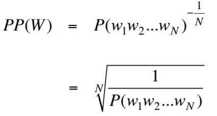
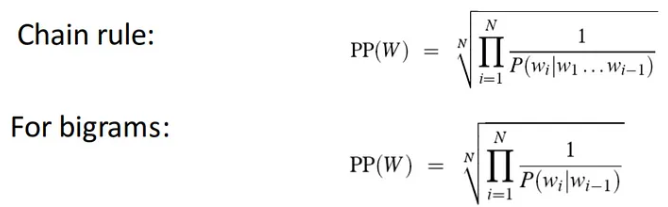
困惑性可以解释为语言模型中分支因素的量度。分支因子代表了给定特定上下文或单词序列的下一个单词或令牌的平均数量。
语言的分支因素是可以遵循任何单词的可能接下来单词的数量。我们可以将困惑视为一种语言的加权平均分支系数。
使用嵌入层和LSTM代码的语言建模是构建和培训语言模型的强大工具。该代码实现结合了自然语言处理中的两个基本组件:嵌入层和长期记忆(LSTM)网络。
嵌入层负责将文本数据转换为分布式表示形式,也称为单词嵌入。这些嵌入捕获单词的语义和句法属性,从而使模型可以理解输入文本的含义和上下文。嵌入层将输入序列中的每个单词映射到高维矢量,该向量是模型中后续层的输入。
代码实现中的LSTM层处理由嵌入层生成的单词嵌入,捕获序列信息并学习文本中的基本模式和结构。
通过组合嵌入层和LSTM网络,该代码可以构建可以生成连贯且上下文适当的文本的语言模型。使用这种方法构建的语言模型可以在大型文本数据集上进行培训,并能够生成现实且有意义的句子,使其成为各种自然语言处理任务的宝贵工具,例如文本生成,机器翻译和情感分析。
此代码实现为基于嵌入层和LSTM架构的构建语言模型提供了简单,清晰和简洁的基础。它是有兴趣探索和尝试最先进的语言建模技术的研究人员,开发人员和爱好者的起点。
通过此代码,您可以更深入地了解嵌入层和LSTM的方式以捕获文本数据中的复杂模式和依赖项。有了这些知识,您可以进一步扩展代码并探索高级技术,例如结合注意机制或变压器体系结构,以增强语言模型的性能和能力。
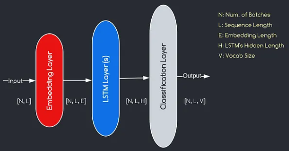
我们将构建的模型对应于上面提供的图表,说明了三个关键组件:嵌入层,LSTM层和分类层。尽管我们已经熟悉LSTM和分类层的目标,但让我们深入研究嵌入层的重要性。
嵌入层通过将表示为索引的每个单词转换为e维数的向量,在模型中起着至关重要的作用。该向量表示允许后续层从输入中学习和提取有意义的信息。值得注意的是,使用索引或单速向量表示单词可能不足,因为他们假设不同单词之间没有关系。
嵌入层进行的映射过程是在训练过程中进行的学习过程。在这个训练阶段,该模型以捕获语义和句法关系的方式将单词与特定向量相关联的能力,从而增强了模型对基本语言结构的理解。
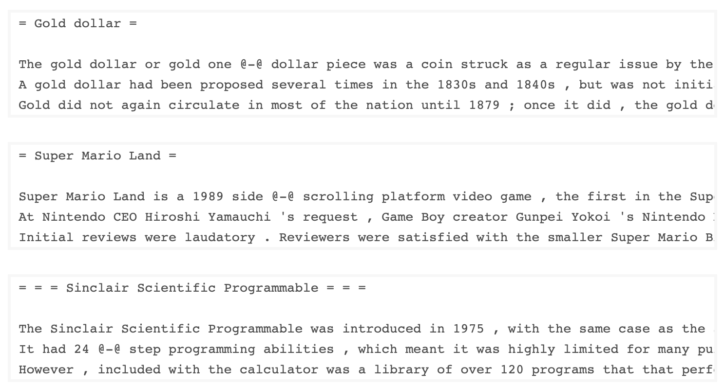
由Salesforce开发的Wkitext-103数据集包含超过1亿个令牌,这些令牌从Wikipedia上的一系列经过验证的商品和精选文章中提取出来。它具有267,340个独特的令牌,在数据集中至少出现3次。由于它具有全长的Wikipedia文章,因此数据集非常适合可以使长期依赖性(例如语言建模)受益的任务。
Wikitext-2数据集是Wikitext-103数据集的一个小版本,因为它仅包含200万个令牌。这个小数据集适用于测试您的语言模型。
该存储库包含用于对UTK数据集执行探索性数据分析的代码,该代码由按年龄,性别和种族分类的图像组成。
要使用TorchText下载数据集,可以使用torchtext.datasets模块。这是如何使用TorchText下载Wikitext-2数据集的示例:
 import torchtext
from torchtext . datasets import WikiText2
data_path = "data"
train_iter , valid_iter , test_iter = WikiText2 ( root = data_path ) 最初,我尝试使用提供的代码来加载Wikitext-2数据集,但遇到了URL的问题(https://s3.amazonaws.com/research.metamind.io/wikite.io/wikite.io/wikitext/wikitext-2-v1.zip)不起作用。为了克服这一点,我决定利用torchtext本库并创建数据集加载程序的自定义实现。
由于原始URL无法正常工作,因此我从GitHub存储库下载了火车,验证和测试数据集,并将其放置在'data/datasets/WikiText2'目录中。
这是代码的细分:
 import os
from typing import Union , Tuple

from torchdata . datapipes . iter import FileOpener , IterableWrapper
from torchtext . data . datasets_utils import _wrap_split_argument , _create_dataset_directory

DATA_DIR = "data"

NUM_LINES = {
    "train" : 36718 ,
    "valid" : 3760 ,
    "test" : 4358 ,
}

DATASET_NAME = "WikiText2"

_EXTRACTED_FILES = {
    "train" : "wiki.train.tokens" ,
    "test" : "wiki.test.tokens" ,
    "valid" : "wiki.valid.tokens" ,
}


def _filepath_fn ( root , split ):
    return os . path . join ( root , _EXTRACTED_FILES [ split ])


@ _create_dataset_directory ( dataset_name = DATASET_NAME )
@ _wrap_split_argument (( "train" , "valid" , "test" ))

def WikiText2 ( root : str , split : Union [ Tuple [ str ], str ]):
    url_dp = IterableWrapper ([ _filepath_fn ( DATA_DIR , split )])
    data_dp = FileOpener ( url_dp , encoding = "utf-8" ). readlines ( strip_newline = False , return_path = False ). shuffle (). set_shuffle ( False ). sharding_filter ()
return data_dp 要使用Wikitext-2数据集加载程序,只需导入Wikitext2函数,然后将其调用所需的数据拆分:
 train_data = WikiText2 ( root = "data/datasets/WikiText2" , split = "train" )
valid_data = WikiText2 ( root = "data/datasets/WikiText2" , split = "valid" )
test_data = WikiText2 ( root = "data/datasets/WikiText2" , split = "test" )该实现的灵感来自官方的TorchText数据集装载机,并利用Torchdata和Torchtext库提供了无缝有效的数据加载体验。
在许多自然语言处理任务中,构建词汇是至关重要的一步,因为它使您可以将单词表示为可以在机器学习模型中使用的唯一标识符。该降价文档演示了如何从一组培训数据中构建词汇并保存以备将来使用。
这是一个函数,封装了构建和保存词汇的过程:
 import torch
from torchtext . data . utils import get_tokenizer
from torchtext . vocab import build_vocab_from_iterator

def build_and_save_vocabulary ( train_iter , vocab_path = 'vocab.pt' , min_freq = 4 ):
    """
    Build a vocabulary from the training data iterator and save it to a file.

    Args:
        train_iter (iterator): An iterator over the training data.
        vocab_path (str, optional): The path to save the vocabulary file. Defaults to 'vocab.pt'.
        min_freq (int, optional): The minimum frequency of a word to be included in the vocabulary. Defaults to 4.

    Returns:
        torchtext.vocab.Vocab: The built vocabulary.
    """
    # Get the tokenizer
    tokenizer = get_tokenizer ( "basic_english" )

    # Build the vocabulary
    vocab = build_vocab_from_iterator ( map ( tokenizer , train_iter ), specials = [ '<unk>' ], min_freq = min_freq )

    # Set the default index to the unknown token
    vocab . set_default_index ( vocab [ '<unk>' ])

    # Save the vocabulary
    torch . save ( vocab , vocab_path )

    return vocab
这是您可以使用此功能的方法:
 # Assuming you have a training data iterator named `train_iter`
vocab = build_and_save_vocabulary ( train_iter , vocab_path = 'my_vocab.pt' )

# You can now use the vocabulary
print ( len ( vocab ))  # 23652
print ( vocab ([ 'ebi' , 'AI' . lower (), 'qwerty' ])) # [0, 1973, 0] build_and_save_vocabulary函数采用三个参数: train_iter (训练数据上的迭代器), vocab_path (保存词汇文件的路径,默认为“ vocab.pt.pt'')和min_freq( min_freq (单词的最小频率都包含在vocabulary中的最小频率,均为4)。basic_english Tokenizer,该函数在英语文本上执行基本令牌化。build_vocab_from_iterator函数来构建词汇,传递训练数据迭代器(后代化后)并指定'<unk>'特殊令牌和最小频率阈值。'<unk>'令牌的ID,这意味着词汇中未找到的任何单词都会映射到未知的令牌上。要使用此功能,您需要拥有一个名为train_iter的培训数据迭代器。然后,您可以调用build_and_save_vocabulary函数,通过train_iter并指定所需的词汇文件路径和最小频率阈值。
该函数将构建词汇,将其保存到指定的文件中,然后返回Vocab对象,然后您可以在下游任务中使用它们。
该代码提供了一种分析Wikitext-2数据集中平均句子长度的方法。这是代码的细分:
 import matplotlib . pyplot as plt

def compute_mean_sentence_length ( data_iter ):
    """
    Computes the mean sentence length for the given data iterator.

    Args:
        data_iter (iterable): An iterable of text data, where each element is a string representing a line of text.

    Returns:
        float: The mean sentence length.
    """
    total_sentence_count = 0
    total_sentence_length = 0

    for line in data_iter :
        sentences = line . split ( '.' )  # Split the line into individual sentences

        for sentence in sentences :
            tokens = sentence . strip (). split ()  # Tokenize the sentence
            sentence_length = len ( tokens )

            if sentence_length > 0 :
                total_sentence_count += 1
                total_sentence_length += sentence_length

    mean_sentence_length = total_sentence_length / total_sentence_count
    return mean_sentence_length

# Compute mean sentence length for each dataset
train_mean = compute_mean_sentence_length ( train_iter )
valid_mean = compute_mean_sentence_length ( valid_iter )
test_mean  = compute_mean_sentence_length ( test_iter )

# Plot the results
datasets = [ 'Train' , 'Valid' , 'Test' ]
means = [ train_mean , valid_mean , test_mean ]

plt . figure ( figsize = ( 6 , 4 ))
plt . bar ( datasets , means )
plt . xlabel ( 'Dataset' )
plt . ylabel ( 'Mean Sentence Length' )
plt . title ( 'Mean Sentence Length in Wikitext-2' )
plt . grid ( True )
plt . show ()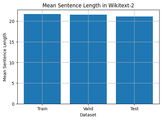
 from collections import Counter

# Compute word frequencies in the training dataset
freqs = Counter ()
for tokens in map ( tokenizer , train_iter ):
    freqs . update ( tokens )

# Find the 10 least common words
least_common_words = freqs . most_common ()[: - 11 : - 1 ]
print ( "Least Common Words:" )
for word , count in least_common_words :
    print ( f" { word } : { count } " )

# Find the 10 most common words
most_common_words = freqs . most_common ( 10 )
print ( " n Most Common Words:" )
for word , count in most_common_words :
print ( f" { word } : { count } " ) from collections import Counter
# Compute word frequencies in the training dataset
freqs = Counter ()
for tokens in map ( tokenizer , train_iter ):
freqs . update ( tokens )
# Count the number of words that repeat 3, 4, and 5 times
count_3 = count_4 = count_5 = 0
for word , freq in freqs . items ():
if freq == 3 :
count_3 += 1
elif freq == 4 :
count_4 += 1
elif freq == 5 :
count_5 += 1
print ( f"Number of words that appear 3 times: { count_3 } " ) # 5130
print ( f"Number of words that appear 4 times: { count_4 } " ) # 3243
print ( f"Number of words that appear 5 times: { count_5 } " ) # 2261 from collections import Counter
import matplotlib . pyplot as plt
# Compute the word lengths in the training dataset
word_lengths = []
for tokens in map ( tokenizer , train_iter ):
word_lengths . extend ( len ( word ) for word in tokens )
# Create a frequency distribution of word lengths
word_length_counts = Counter ( word_lengths )
# Plot the word length distribution
plt . figure ( figsize = ( 10 , 6 ))
plt . bar ( word_length_counts . keys (), word_length_counts . values ())
plt . xlabel ( "Word Length" )
plt . ylabel ( "Frequency" )
plt . title ( "Word Length Distribution in Wikitext-2 Dataset" )
plt . show ()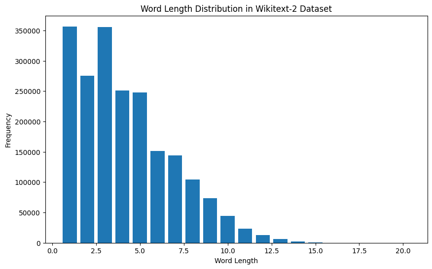
 import spacy
import en_core_web_sm

# Load the small English language model from SpaCy
nlp = spacy . load ( "en_core_web_sm" )

# Alternatively, you can use the en_core_web_sm module to load the model
nlp = en_core_web_sm . load ()

# Process the given sentence using the loaded language model
doc = nlp ( "This is a sentence." )

# Print the text and part-of-speech tag for each token in the sentence
print ([( w . text , w . pos_ ) for w in doc ])

# [('This', 'PRON'), ('is', 'AUX'), ('a', 'DET'), ('sentence', 'NOUN'), ('.', 'PUNCT')]
对于Wikitext-2数据集:
 import spacy

# Load the English language model
nlp = spacy . load ( "en_core_web_sm" )

# Perform POS tagging on the training dataset
pos_tags = []
for tokens in map ( tokenizer , train_iter ):
    doc = nlp ( " " . join ( tokens ))
    pos_tags . extend ([( token . text , token . pos_ ) for token in doc ])

# Count the frequency of each POS tag
pos_tag_counts = Counter ( tag for _ , tag in pos_tags )

# Print the most common POS tags
print ( "Most Common Part-of-Speech Tags:" )
for tag , count in pos_tag_counts . most_common ( 10 ):
    print ( f" { tag } : { count } " )

# Visualize the POS tag distribution
plt . figure ( figsize = ( 12 , 6 ))
plt . bar ( pos_tag_counts . keys (), pos_tag_counts . values ())
plt . xticks ( rotation = 90 )
plt . xlabel ( "Part-of-Speech Tag" )
plt . ylabel ( "Frequency" )
plt . title ( "Part-of-Speech Tag Distribution in Wikitext-2 Dataset" )
plt . show ()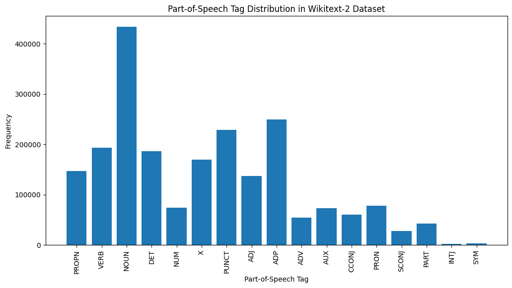
这是对提供的输出中最常见的POS标签的简要说明:
名词:名词代表人,地方,事物或想法。
ADP :使用介词和后置诸如介词,用于表达单词或短语之间的关系。
标点:标点符号,这对于分离和结构句子和文字至关重要。
动词:动词描述文本中的动作,状态或事件。
DET :确定词,例如文章(例如,“ the,” a,“”),提供了有关名词的其他信息。
X :此标签通常用于外语单词,缩写或其他不适合标准POS类别的特定语言令牌。
提示:代表人物,地点,组织或其他实体的特定名称的专有名词。
adj :形容词修改或描述名词和代词。
pron :代词代替名词,使文本更简洁,重复性较低。
数字:代表数量,日期或其他数值信息的数字。
POS标签的这种分布可以提供有关文本的语言特征的见解,例如名词的优势,apositions的普遍性或适当名词的使用,这可能有助于文本分类,信息提取或设式分析等任务。
 import spacy
import matplotlib . pyplot as plt

# Load the English language model
nlp = spacy . load ( "en_core_web_sm" )

# Perform NER on the training dataset
named_entities = []
for tokens in map ( tokenizer , train_iter ):
    doc = nlp ( " " . join ( tokens ))
    named_entities . extend ([( ent . text , ent . label_ ) for ent in doc . ents ])

# Count the frequency of each named entity type
ner_counts = Counter ( label for _ , label in named_entities )

# Print the most common named entity types
print ( "Most Common Named Entity Types:" )
for label , count in ner_counts . most_common ( 10 ):
    print ( f" { label } : { count } " )

# Visualize the named entity distribution
plt . figure ( figsize = ( 12 , 6 ))
plt . bar ( ner_counts . keys (), ner_counts . values ())
plt . xticks ( rotation = 90 )
plt . xlabel ( "Named Entity Type" )
plt . ylabel ( "Frequency" )
plt . title ( "Named Entity Distribution in Wikitext-2 Dataset" )
plt . show ()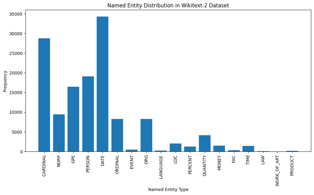
Here's a brief explanation of the most common named entity types in the output:
DATE : Represents specific dates, time periods, or temporal expressions, such as "June 15, 2024" or "last year".
CARDINAL : Includes numerical values, such as quantities, ages, or measurements.
PERSON : Identifies the names of individual people.
GPE (Geopolitical Entity): This entity type represents named geographical locations, such as countries, cities, or states.
NORP (Nationalities, Religious, or Political Groups): This entity type includes named groups or affiliations based on nationality, religion, or political ideology.
ORDINAL : Represents ordinal numbers, such as "first," "second," or "3rd".
ORG (Organization): The names of companies, institutions, or other organized groups.
QUANTITY : Includes non-numeric quantities, such as "a few" or "several".
LOC (Location): Represents named geographical locations, such as continents, regions, or landforms.
MONEY : Identifies monetary values, such as dollar amounts or currency names.
This distribution of named entity types can provide valuable insights into the content and focus of the text. For example, the prominence of DATE and CARDINAL entities may suggest a text that deals with numerical or temporal information, while the prevalence of PERSON, ORG, and GPE entities could indicate a text that discusses people, organizations, and geographical locations.
Understanding the named entity distribution can be useful in a variety of applications, such as information extraction, question answering, and text summarization, where identifying and categorizing key named entities is crucial for understanding the context and content of the text.
 from wordcloud import WordCloud
import matplotlib . pyplot as plt

# Load the training dataset
with open ( "data/wiki.train.tokens" , "r" ) as f :
    train_text = f . read (). split ()

# Create a string from the entire training dataset
text = " " . join ( train_text )

# Generate the word cloud
wordcloud = WordCloud ( width = 800 , height = 400 , background_color = 'white' ). generate ( text )

# Plot the word cloud
plt . figure ( figsize = ( 12 , 8 ))
plt . imshow ( wordcloud , interpolation = 'bilinear' )
plt . axis ( 'off' )
plt . title ( 'Word Cloud for Wikitext-2 Training Dataset' )
plt . show ()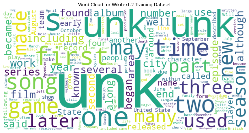
 from sentence_transformers import SentenceTransformer
from sklearn . cluster import KMeans
from collections import defaultdict
from wordcloud import WordCloud
import matplotlib . pyplot as plt

# Load the BERT-based sentence transformer model
model = SentenceTransformer ( 'bert-base-nli-mean-tokens' )

# Load the training dataset
with open ( "data/wiki.valid.tokens" , "r" ) as f :
    train_text = f . read (). split ()

# Compute the BERT embeddings for each unique word in the dataset
unique_words = set ( train_text )
word_embeddings = model . encode ( list ( unique_words ))

# Cluster the words using K-Means
num_clusters = 5
kmeans = KMeans ( n_clusters = num_clusters , random_state = 42 )
clusters = kmeans . fit_predict ( word_embeddings )

# Group the words by cluster
word_clusters = defaultdict ( list )
for i , word in enumerate ( unique_words ):
    word_clusters [ clusters [ i ]]. append ( word )

# Create a word cloud for each cluster
fig , axes = plt . subplots ( 1 , 5 , figsize = ( 14 , 12 ))
axes = axes . flatten ()

for cluster_id , cluster_words in word_clusters . items ():
    word_cloud = WordCloud ( width = 400 , height = 200 , background_color = 'white' ). generate ( ' ' . join ( cluster_words ))
    axes [ cluster_id ]. imshow ( word_cloud , interpolation = 'bilinear' )
    axes [ cluster_id ]. set_title ( f"Cluster { cluster_id } " )
    axes [ cluster_id ]. axis ( 'off' )

plt . subplots_adjust ( wspace = 0.4 , hspace = 0.6 )

plt . tight_layout ()
plt . show ()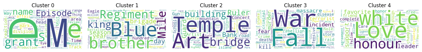
The two data formats, N x B x L and M x L , are commonly used in language modeling tasks, particularly in the context of neural network-based models.
N x B x L format:
N represents the number of batches. In this case, the dataset is divided into N smaller batches, which is a common practice to improve the efficiency and stability of the training process.B is the batch size, which represents the number of samples (eg, sentences, paragraphs, or documents) within each batch.L is the length of a sample within each batch, which typically corresponds to the number of tokens (words) in a sample. M x L format:
N x B x L format.M is equal to N x B , which represents the total number of samples (eg, sentences, paragraphs, or documents) in the dataset.L is the length of each sample, which corresponds to the number of tokens (words) in the sample. The choice between these two formats depends on the specific requirements of your language modeling task and the capabilities of the neural network architecture you're working with. If you're training a neural network-based language model, the N x B x L format is typically preferred, as it allows for efficient batch-based training and can lead to faster convergence and better performance. However, if your task doesn't involve neural networks or if the dataset is relatively small, the M x L format may be more suitable.
 def prepare_language_model_data ( raw_text_iterator , sequence_length ):
    """
    Prepare PyTorch tensors for a language model.

    Args:
        raw_text_iterator (iterable): An iterator of raw text data.
        sequence_length (int): The length of the input and target sequences.

    Returns:
        tuple: A tuple containing two PyTorch tensors:
            - inputs (torch.Tensor): A tensor of input sequences.
            - targets (torch.Tensor): A tensor of target sequences.
    """
    # Convert the raw text iterator into a single PyTorch tensor
    data = torch . cat ([ torch . LongTensor ( vocab ( tokenizer ( line ))) for line in raw_text_iterator ])

    # Calculate the number of complete sequences that can be formed
    num_sequences = len ( data ) // sequence_length

    # Calculate the remainder of the data length divided by the sequence length
    remainder = len ( data ) % sequence_length

    # If the remainder is 0, add a single <unk> token to the end of the data tensor
    if remainder == 0 :
        unk_tokens = torch . LongTensor ([ vocab [ '<unk>' ]])
        data = torch . cat ([ data , unk_tokens ])

    # Extract the input and target sequences from the data tensor
    inputs = data [: num_sequences * sequence_length ]. reshape ( - 1 , sequence_length )
    targets = data [ 1 : num_sequences * sequence_length + 1 ]. reshape ( - 1 , sequence_length )

    print ( len ( inputs ), len ( targets ))
return inputs , targets sequence_length = 30
X_train , y_train = prepare_language_model_data ( train_iter , sequence_length )
X_valid , y_valid = prepare_language_model_data ( valid_iter , sequence_length )
X_test , y_test = prepare_language_model_data ( test_iter , sequence_length )
X_train . shape , y_train . shape , X_valid . shape , y_valid . shape , X_test . shape , y_test . shape
( torch . Size ([ 68333 , 30 ]),
torch . Size ([ 68333 , 30 ]),
torch . Size ([ 7147 , 30 ]),
torch . Size ([ 7147 , 30 ]),
torch . Size ([ 8061 , 30 ]),
torch . Size ([ 8061 , 30 ])) This code defines a PyTorch Dataset class for working with language model data. The LanguageModelDataset class takes in input and target tensors and provides the necessary methods for accessing the data.
 class LanguageModelDataset ( Dataset ):
    def __init__ ( self , inputs , targets ):
        self . inputs = inputs
        self . targets = targets

    def __len__ ( self ):
        return self . inputs . shape [ 0 ]

    def __getitem__ ( self , idx ):
return self . inputs [ idx ], self . targets [ idx ]The LanguageModelDataset class can be used as follows:
 # Create the datasets
train_set = LanguageModelDataset ( X_train , y_train )
valid_set = LanguageModelDataset ( X_valid , y_valid )
test_set  = LanguageModelDataset ( X_test , y_test )

# Create data loaders (optional)
train_loader = DataLoader ( train_set , batch_size = 32 , shuffle = True )
valid_loader = DataLoader ( valid_set , batch_size = 32 )
test_loader  = DataLoader ( test_set , batch_size = 32 )

# Access the data
x_batch , y_batch = next ( iter ( train_loader ))
print ( f"Input batch shape: { x_batch . shape } " )  # Input batch shape: torch.Size([32, 30])
print ( f"Target batch shape: { y_batch . shape } " ) # Target batch shape: torch.Size([32, 30]) The code defines a custom PyTorch language model that allows you to use different types of word embeddings, including randomly initialized embeddings, pre-trained GloVe embeddings, pre-trained FastText embeddings, by simply specifying the embedding_type argument when creating the model instance.
 import torch . nn as nn
from torchtext . vocab import GloVe , FastText


class LanguageModel ( nn . Module ):
    def __init__ ( self , vocab_size , embedding_dim ,
                 hidden_dim , num_layers , dropout_embd = 0.5 ,
                 dropout_rnn = 0.5 , embedding_type = 'random' ):

        super (). __init__ ()
        self . num_layers = num_layers
        self . hidden_dim = hidden_dim
        self . embedding_dim = embedding_dim
        self . embedding_type = embedding_type

        if embedding_type == 'random' :
            self . embedding = nn . Embedding ( vocab_size , embedding_dim )
            self . embedding . weight . data . uniform_ ( - 0.1 , 0.1 )

        elif embedding_type == 'glove' :
            self . glove = GloVe ( name = '6B' , dim = embedding_dim )
            self . embedding = nn . Embedding ( vocab_size , embedding_dim )
            self . embedding . weight . data . copy_ ( self . glove . vectors )
            self . embedding . weight . requires_grad = False

        elif embedding_type == 'fasttext' :
            self . glove = FastText ( language = 'en' )
            self . embedding = nn . Embedding ( vocab_size , embedding_dim )
            self . embedding . weight . data . copy_ ( self . fasttext . vectors )
            self . embedding . weight . requires_grad = False

        else :
            raise ValueError ( "Invalid embedding_type. Choose from 'random', 'glove', 'fasttext'." )

        self . dropout = nn . Dropout ( p = dropout_embd )
        self . lstm = nn . LSTM ( embedding_dim , hidden_dim , num_layers = num_layers ,
                           dropout = dropout_rnn , batch_first = True )
        self . fc = nn . Linear ( hidden_dim , vocab_size )

    def forward ( self , src ):
        embedding = self . dropout ( self . embedding ( src ))
        output , hidden = self . lstm ( embedding )
        prediction = self . fc ( output )
return prediction model = LanguageModel ( vocab_size = len ( vocab ),
embedding_dim = 300 ,
hidden_dim = 512 ,
num_layers = 2 ,
dropout_embd = 0.65 ,
dropout_rnn = 0.5 ,
embedding_type = 'glove' ) def num_trainable_params ( model ):
nums = sum ( p . numel () for p in model . parameters () if p . requires_grad ) / 1e6
return nums
# Calculate the number of trainable parameters in the embedding, LSTM, and fully connected layers of the LanguageModel instance 'model'
num_trainable_params ( model . embedding ) # (7.0956)
num_trainable_params ( model . lstm ) # (3.76832)
num_trainable_params ( model . fc ) # (12.133476)

