food 101 keras
1.0.0
 from IPython . display import HTML , Image

url = 'http://stratospark.com/demos/food-101/'
el = '<' + 'iframe src="{}"' . format ( url ) + ' width="100%" height=600></iframe>' # prevent notebook render bug
HTML ( el )Если вы читаете это на GitHub, демонстрация выглядит так. Пожалуйста, перейдите по ссылке ниже, чтобы просмотреть демонстрацию в прямом эфире в моем блоге.
Image ( 'demo.jpg' )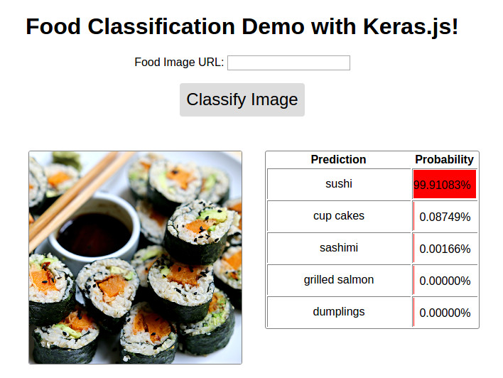
Демо, доступная @ http://blog.stratospark.com/deep-learning-applied-food-classiation-deep-learning-keras.html
Код доступен @ https://github.com/stratospark/food-101-keras
Обновления
Свещательные нейронные сети (CNN), методика в более широкой области глубокого обучения, были революционной силой в приложениях компьютерного зрения, особенно в последние полдесятилетние или около того. Одним из основных вариантов использования является классификация изображений, например, определяет, является ли картина собаки или кошки.
Вам не нужно ограничивать себя бинарным классификатором, конечно; CNN могут легко масштабироваться до тысяч различных классов, как видно из хорошо известного набора данных ImageNet 1000 классов, используемых для оценки производительности алгоритма компьютерного зрения.
За последние пару лет эти передовые методы стали доступны для более широкого сообщества разработки программного обеспечения. Пакеты промышленности, такие как Tensorflow, дали нам те же строительные блоки, которые Google использует для написания приложений глубокого обучения для встроенных/мобильных устройств для масштабируемых кластеров в облаке - без необходимости ручной кодики операций матрицы графического процессора, градиентов частичных производных и стохастических оптимизаторов. Это делает возможным эффективное применение.
Помимо всего этого, являются удобными API, такие как кера, которые абстрагируют некоторые детали нижнего уровня и позволяют нам сосредоточиться на быстрого прототипирования графика вычисления глубокого обучения. Как будто мы смешали и сопоставляли Legos, чтобы получить желаемый результат.
Как вступительный проект для себя, я решил использовать предварительно обученный классификатор изображений, который поставляется с керами, и перепровею его в наборе данных, который мне кажется интересным. Я очень увлекаюсь хорошей едой и домашней кухней, так что что -то в этом роде было аппетитным.
В статье, Food-101-дискриминационные компоненты добычи полезных ископаемых со случайными лесами, они вводят набор данных Food-101. Существует 101 различные классы пищи, с 1000 маркированными изображениями на класс, доступные для контролируемого обучения.
Я был вдохновлен этим сообщением в блоге Keras: создание мощных моделей классификации изображений с использованием очень мало данных и связанный сценарий, который я нашел на Github: Keras-Finetuning.
Я недавно построил систему с целью экспериментов с глубоким обучением. Ключевыми компонентами являются Nvidia Titan X Pascal с 12 ГБ памяти, 96 ГБ системной оперативной памяти, а также 12-ядерный Intel Core i7. Он работает 64-битный Ubuntu 16.04 и использует распределение Anaconda Python. К сожалению, вы не сможете следовать вместе с этим ноутбуком в своей собственной системе, если у вас не будет достаточно оперативной памяти. В будущем я хотел бы научиться обращаться с наборами данных о большей, чем RAM, работающими. Пожалуйста, свяжитесь с нами, если у вас есть идеи!
Я потратил около 1 месяца на строительство этого проекта, пытаясь обучить десятки моделей и исследовать различные области, такие как многопроцессорная передача для более быстрого увеличения изображения. Это очищенная версия ноутбука, которая содержит мою лучшую модель выполнения по состоянию на 22 января 2017 года.
После тонкой настройки модели Google PesceptV3 я смог достичь около 82,03% Топ-1 на тестовом наборе с использованием одного урожая на элемент. Используя 10 сельскохозяйственных культур в пример и, принимая наиболее частый прогнозируемый класс (ES), я смог достичь 86,97% Топ-1 и точность 97,42% топ-5 топ-5
Другие смогли достичь более точных результатов:
Реализовано! Проверьте: http://blog.stratospark.com/creating-a-deep-learning-ios-app-with-keras-and-tensorflow.html
Давайте импортируем все пакеты, необходимые для остальной части записной книжки:
 import matplotlib . pyplot as plt
import matplotlib . image as img
import numpy as np
from scipy . misc import imresize

% matplotlib inline

import os
from os import listdir
from os . path import isfile , join
import shutil
import stat
import collections
from collections import defaultdict

from ipywidgets import interact , interactive , fixed
import ipywidgets as widgets

import h5py
from sklearn . model_selection import train_test_split
from keras . utils . np_utils import to_categorical
from keras . applications . inception_v3 import preprocess_input
from keras . models import load_model
Using TensorFlow backend.
Загрузите набор данных и извлеките его в папку ноутбука. Это может быть проще сделать в отдельном окне терминала.
# !wget http://data.vision.ee.ethz.ch/cvl/food-101.tar.gz # !tar xzvf food-101.tar.gzПосмотрим, какие продукты представлены здесь:
!l s food - 101 / images apple_pie eggs_benedict onion_rings
baby_back_ribs escargots oysters
baklava falafel pad_thai
beef_carpaccio filet_mignon paella
beef_tartare fish_and_chips pancakes
beet_salad foie_gras panna_cotta
beignets french_fries peking_duck
bibimbap french_onion_soup pho
bread_pudding french_toast pizza
breakfast_burrito fried_calamari pork_chop
bruschetta fried_rice poutine
caesar_salad frozen_yogurt prime_rib
cannoli garlic_bread pulled_pork_sandwich
caprese_salad gnocchi ramen
carrot_cake greek_salad ravioli
ceviche grilled_cheese_sandwich red_velvet_cake
cheesecake grilled_salmon risotto
cheese_plate guacamole samosa
chicken_curry gyoza sashimi
chicken_quesadilla hamburger scallops
chicken_wings hot_and_sour_soup seaweed_salad
chocolate_cake hot_dog shrimp_and_grits
chocolate_mousse huevos_rancheros spaghetti_bolognese
churros hummus spaghetti_carbonara
clam_chowder ice_cream spring_rolls
club_sandwich lasagna steak
crab_cakes lobster_bisque strawberry_shortcake
creme_brulee lobster_roll_sandwich sushi
croque_madame macaroni_and_cheese tacos
cup_cakes macarons takoyaki
deviled_eggs miso_soup tiramisu
donuts mussels tuna_tartare
dumplings nachos waffles
edamame omelette
!l s food - 101 / images / apple_pie / | head - 10 1005649.jpg
1011328.jpg
101251.jpg
1014775.jpg
1026328.jpg
1028787.jpg
1034399.jpg
103801.jpg
1038694.jpg
1043283.jpg
ls: write error: Broken pipe
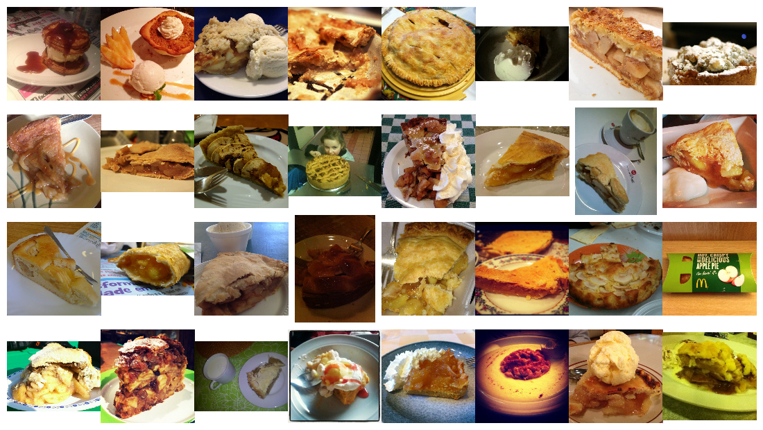
Давайте посмотрим на некоторые случайные изображения из каждого класса продуктов питания. Вы можете щелкнуть правой кнопкой мыши и открыть изображение в новом окне или сохранить его, чтобы увидеть его в более высоком разрешении.
 root_dir = 'food-101/images/'
rows = 17
cols = 6
fig , ax = plt . subplots ( rows , cols , frameon = False , figsize = ( 15 , 25 ))
fig . suptitle ( 'Random Image from Each Food Class' , fontsize = 20 )
sorted_food_dirs = sorted ( os . listdir ( root_dir ))
for i in range ( rows ):
    for j in range ( cols ):
        try :
            food_dir = sorted_food_dirs [ i * cols + j ]
        except :
            break
        all_files = os . listdir ( os . path . join ( root_dir , food_dir ))
        rand_img = np . random . choice ( all_files )
        img = plt . imread ( os . path . join ( root_dir , food_dir , rand_img ))
        ax [ i ][ j ]. imshow ( img )
        ec = ( 0 , .6 , .1 )
        fc = ( 0 , .7 , .2 )
        ax [ i ][ j ]. text ( 0 , - 20 , food_dir , size = 10 , rotation = 0 ,
                ha = "left" , va = "top" ,
                bbox = dict ( boxstyle = "round" , ec = ec , fc = fc ))
plt . setp ( ax , xticks = [], yticks = [])
plt . tight_layout ( rect = [ 0 , 0.03 , 1 , 0.95 ])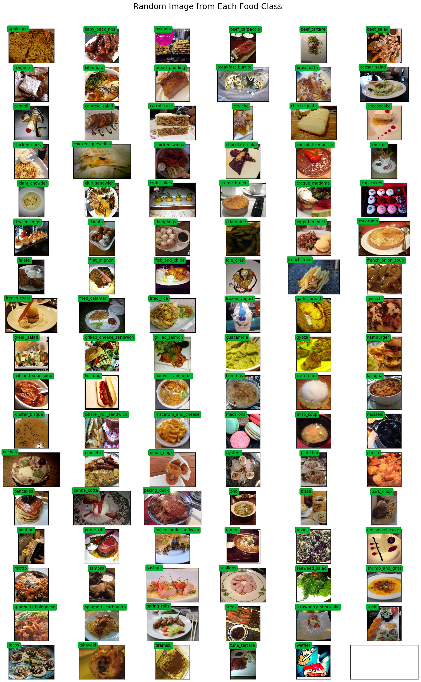
multiprocessing.Pool .
 # Setup multiprocessing pool
# Do this early, as once images are loaded into memory there will be Errno 12
# http://stackoverflow.com/questions/14749897/python-multiprocessing-memory-usage
import multiprocessing as mp

num_processes = 6
pool = mp . Pool ( processes = num_processes )
Нам нужны карты от класса до индекса и наоборот, для правильной кодировки метки и красивой печати.
 class_to_ix = {}
ix_to_class = {}
with open ( 'food-101/meta/classes.txt' , 'r' ) as txt :
    classes = [ l . strip () for l in txt . readlines ()]
    class_to_ix = dict ( zip ( classes , range ( len ( classes ))))
    ix_to_class = dict ( zip ( range ( len ( classes )), classes ))
    class_to_ix = { v : k for k , v in ix_to_class . items ()}
sorted_class_to_ix = collections . OrderedDict ( sorted ( class_to_ix . items ()))
Набор данных Food-101 имеет предоставленное разделение поездов/тестирования. Мы хотим использовать это, чтобы сравнить нашу эффективность классификации с другими реализациями.
 # Only split files if haven't already
if not os . path . isdir ( './food-101/test' ) and not os . path . isdir ( './food-101/train' ):

    def copytree ( src , dst , symlinks = False , ignore = None ):
        if not os . path . exists ( dst ):
            os . makedirs ( dst )
            shutil . copystat ( src , dst )
        lst = os . listdir ( src )
        if ignore :
            excl = ignore ( src , lst )
            lst = [ x for x in lst if x not in excl ]
        for item in lst :
            s = os . path . join ( src , item )
            d = os . path . join ( dst , item )
            if symlinks and os . path . islink ( s ):
                if os . path . lexists ( d ):
                    os . remove ( d )
                os . symlink ( os . readlink ( s ), d )
                try :
                    st = os . lstat ( s )
                    mode = stat . S_IMODE ( st . st_mode )
                    os . lchmod ( d , mode )
                except :
                    pass # lchmod not available
            elif os . path . isdir ( s ):
                copytree ( s , d , symlinks , ignore )
            else :
                shutil . copy2 ( s , d )

    def generate_dir_file_map ( path ):
        dir_files = defaultdict ( list )
        with open ( path , 'r' ) as txt :
            files = [ l . strip () for l in txt . readlines ()]
            for f in files :
                dir_name , id = f . split ( '/' )
                dir_files [ dir_name ]. append ( id + '.jpg' )
        return dir_files

    train_dir_files = generate_dir_file_map ( 'food-101/meta/train.txt' )
    test_dir_files = generate_dir_file_map ( 'food-101/meta/test.txt' )


    def ignore_train ( d , filenames ):
        print ( d )
        subdir = d . split ( '/' )[ - 1 ]
        to_ignore = train_dir_files [ subdir ]
        return to_ignore

    def ignore_test ( d , filenames ):
        print ( d )
        subdir = d . split ( '/' )[ - 1 ]
        to_ignore = test_dir_files [ subdir ]
        return to_ignore

    copytree ( 'food-101/images' , 'food-101/test' , ignore = ignore_train )
    copytree ( 'food-101/images' , 'food-101/train' , ignore = ignore_test )

else :
    print ( 'Train/Test files already copied into separate folders.' )
Train/Test files already copied into separate folders.
Теперь мы готовы загрузить обучение и тестирование изображений в память. После того, как все будет загружено, будет выделено около 80 ГБ памяти.
Любые изображения, которые имеют ширину или длину меньше, чем min_size будут изменены. Это так, что мы можем взять культуру правильного размера во время увеличения изображения.
 % % time

# Load dataset images and resize to meet minimum width and height pixel size
def load_images ( root , min_side = 299 ):
    all_imgs = []
    all_classes = []
    resize_count = 0
    invalid_count = 0
    for i , subdir in enumerate ( listdir ( root )):
        imgs = listdir ( join ( root , subdir ))
        class_ix = class_to_ix [ subdir ]
        print ( i , class_ix , subdir )
        for img_name in imgs :
            img_arr = img . imread ( join ( root , subdir , img_name ))
            img_arr_rs = img_arr
            try :
                w , h , _ = img_arr . shape
                if w < min_side :
                    wpercent = ( min_side / float ( w ))
                    hsize = int (( float ( h ) * float ( wpercent )))
                    #print('new dims:', min_side, hsize)
                    img_arr_rs = imresize ( img_arr , ( min_side , hsize ))
                    resize_count += 1
                elif h < min_side :
                    hpercent = ( min_side / float ( h ))
                    wsize = int (( float ( w ) * float ( hpercent )))
                    #print('new dims:', wsize, min_side)
                    img_arr_rs = imresize ( img_arr , ( wsize , min_side ))
                    resize_count += 1
                all_imgs . append ( img_arr_rs )
                all_classes . append ( class_ix )
            except :
                print ( 'Skipping bad image: ' , subdir , img_name )
                invalid_count += 1
    print ( len ( all_imgs ), 'images loaded' )
    print ( resize_count , 'images resized' )
    print ( invalid_count , 'images skipped' )
    return np . array ( all_imgs ), np . array ( all_classes )

X_test , y_test = load_images ( 'food-101/test' , min_side = 299 )
0 41 french_onion_soup
1 99 tuna_tartare
2 2 baklava
3 12 cannoli
4 8 bread_pudding
5 58 ice_cream
6 63 macarons
7 38 fish_and_chips
8 3 beef_carpaccio
9 59 lasagna
10 84 risotto
11 53 hamburger
12 7 bibimbap
13 15 ceviche
14 92 spring_rolls
15 78 poutine
16 76 pizza
17 19 chicken_quesadilla
18 71 paella
19 11 caesar_salad
20 30 deviled_eggs
21 40 french_fries
22 25 club_sandwich
23 77 pork_chop
24 31 donuts
25 93 steak
26 43 fried_calamari
27 52 gyoza
28 20 chicken_wings
29 47 gnocchi
30 46 garlic_bread
31 81 ramen
32 86 sashimi
33 100 waffles
34 60 lobster_bisque
35 23 churros
36 1 baby_back_ribs
37 0 apple_pie
38 27 creme_brulee
39 79 prime_rib
40 54 hot_and_sour_soup
41 55 hot_dog
42 82 ravioli
43 66 nachos
44 85 samosa
45 95 sushi
46 70 pad_thai
47 87 scallops
48 42 french_toast
49 13 caprese_salad
50 21 chocolate_cake
51 83 red_velvet_cake
52 88 seaweed_salad
53 96 tacos
54 16 cheesecake
55 90 spaghetti_bolognese
56 94 strawberry_shortcake
57 64 miso_soup
58 98 tiramisu
59 74 peking_duck
60 17 cheese_plate
61 69 oysters
62 14 carrot_cake
63 6 beignets
64 61 lobster_roll_sandwich
65 45 frozen_yogurt
66 24 clam_chowder
67 9 breakfast_burrito
68 72 pancakes
69 32 dumplings
70 57 hummus
71 10 bruschetta
72 44 fried_rice
73 97 takoyaki
74 50 grilled_salmon
75 4 beef_tartare
76 89 shrimp_and_grits
77 28 croque_madame
78 49 grilled_cheese_sandwich
79 80 pulled_pork_sandwich
80 56 huevos_rancheros
81 35 escargots
82 91 spaghetti_carbonara
83 34 eggs_benedict
84 33 edamame
85 22 chocolate_mousse
86 18 chicken_curry
87 65 mussels
88 36 falafel
89 37 filet_mignon
90 26 crab_cakes
91 48 greek_salad
92 5 beet_salad
93 51 guacamole
94 29 cup_cakes
95 68 onion_rings
96 39 foie_gras
97 67 omelette
98 73 panna_cotta
99 75 pho
100 62 macaroni_and_cheese
25250 images loaded
693 images resized
0 images skipped
CPU times: user 1min 18s, sys: 4.82 s, total: 1min 23s
Wall time: 1min 23s
 % % time
X_train , y_train = load_images ( 'food-101/train' , min_side = 299 )
0 41 french_onion_soup
1 99 tuna_tartare
2 2 baklava
3 12 cannoli
4 8 bread_pudding
Skipping bad image: bread_pudding 1375816.jpg
5 58 ice_cream
6 63 macarons
7 38 fish_and_chips
8 3 beef_carpaccio
9 59 lasagna
Skipping bad image: lasagna 3787908.jpg
10 84 risotto
11 53 hamburger
12 7 bibimbap
13 15 ceviche
14 92 spring_rolls
15 78 poutine
16 76 pizza
17 19 chicken_quesadilla
18 71 paella
19 11 caesar_salad
20 30 deviled_eggs
21 40 french_fries
22 25 club_sandwich
23 77 pork_chop
24 31 donuts
25 93 steak
Skipping bad image: steak 1340977.jpg
26 43 fried_calamari
27 52 gyoza
28 20 chicken_wings
29 47 gnocchi
30 46 garlic_bread
31 81 ramen
32 86 sashimi
33 100 waffles
34 60 lobster_bisque
35 23 churros
36 1 baby_back_ribs
37 0 apple_pie
38 27 creme_brulee
39 79 prime_rib
40 54 hot_and_sour_soup
41 55 hot_dog
42 82 ravioli
43 66 nachos
44 85 samosa
45 95 sushi
46 70 pad_thai
47 87 scallops
48 42 french_toast
49 13 caprese_salad
50 21 chocolate_cake
51 83 red_velvet_cake
52 88 seaweed_salad
53 96 tacos
54 16 cheesecake
55 90 spaghetti_bolognese
56 94 strawberry_shortcake
57 64 miso_soup
58 98 tiramisu
59 74 peking_duck
60 17 cheese_plate
61 69 oysters
62 14 carrot_cake
63 6 beignets
64 61 lobster_roll_sandwich
65 45 frozen_yogurt
66 24 clam_chowder
67 9 breakfast_burrito
68 72 pancakes
69 32 dumplings
70 57 hummus
71 10 bruschetta
72 44 fried_rice
73 97 takoyaki
74 50 grilled_salmon
75 4 beef_tartare
76 89 shrimp_and_grits
77 28 croque_madame
78 49 grilled_cheese_sandwich
79 80 pulled_pork_sandwich
80 56 huevos_rancheros
81 35 escargots
82 91 spaghetti_carbonara
83 34 eggs_benedict
84 33 edamame
85 22 chocolate_mousse
86 18 chicken_curry
87 65 mussels
88 36 falafel
89 37 filet_mignon
90 26 crab_cakes
91 48 greek_salad
92 5 beet_salad
93 51 guacamole
94 29 cup_cakes
95 68 onion_rings
96 39 foie_gras
97 67 omelette
98 73 panna_cotta
99 75 pho
100 62 macaroni_and_cheese
75747 images loaded
2091 images resized
3 images skipped
CPU times: user 3min 51s, sys: 13.9 s, total: 4min 5s
Wall time: 4min 5s
 print ( 'X_train shape' , X_train . shape )
print ( 'y_train shape' , y_train . shape )
print ( 'X_test shape' , X_test . shape )
print ( 'y_test shape' , y_test . shape )
X_train shape (75747,)
y_train shape (75747,)
X_test shape (25250,)
y_test shape (25250,)
@ interact ( n = ( 0 , len ( X_train )))
def show_pic ( n ):
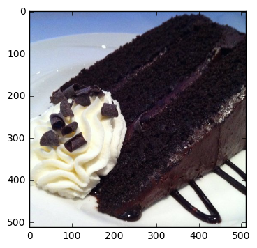
plt . imshow ( X_train [ n ])
print ( 'class:' , y_train [ n ], ix_to_class [ y_train [ n ]]) class: 21 chocolate_cake
@ interact ( n = ( 0 , len ( X_test )))
def show_pic ( n ):
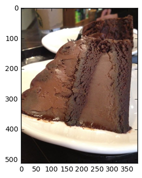
plt . imshow ( X_test [ n ])
print ( 'class:' , y_test [ n ], ix_to_class [ y_test [ n ]]) class: 21 chocolate_cake
 @ interact ( n_class = sorted_class_to_ix )
def show_random_images_of_class ( n_class = 0 ):
    print ( n_class )
    nrows = 4
    ncols = 8
    fig , axes = plt . subplots ( nrows = nrows , ncols = ncols )
    fig . set_size_inches ( 12 , 8 )
    #fig.tight_layout()
    imgs = np . random . choice (( y_train == n_class ). nonzero ()[ 0 ], nrows * ncols )
    for i , ax in enumerate ( axes . flat ):
        im = ax . imshow ( X_train [ imgs [ i ]])
        ax . set_axis_off ()
        ax . title . set_visible ( False )
        ax . xaxis . set_ticks ([])
        ax . yaxis . set_ticks ([])
        for spine in ax . spines . values ():
            spine . set_visible ( False )
    plt . subplots_adjust ( left = 0 , wspace = 0 , hspace = 0 )
    plt . show ()
0
 @ interact ( n_class = sorted_class_to_ix )
def show_random_images_of_class ( n_class = 0 ):
    print ( n_class )
    nrows = 4
    ncols = 8
    fig , axes = plt . subplots ( nrows = nrows , ncols = ncols )
    fig . set_size_inches ( 12 , 8 )
    #fig.tight_layout()
    imgs = np . random . choice (( y_test == n_class ). nonzero ()[ 0 ], nrows * ncols )
    for i , ax in enumerate ( axes . flat ):
        im = ax . imshow ( X_test [ imgs [ i ]])
        ax . set_axis_off ()
        ax . title . set_visible ( False )
        ax . xaxis . set_ticks ([])
        ax . yaxis . set_ticks ([])
        for spine in ax . spines . values ():
            spine . set_visible ( False )
    plt . subplots_adjust ( left = 0 , wspace = 0 , hspace = 0 )
    plt . show ()
0
Нам необходимо одноказкое кодировать каждую значение метки, чтобы создать вектор двоичных функций, а не одну функцию, которая может принять значения n_classes .
 from keras . utils . np_utils import to_categorical

n_classes = 101
y_train_cat = to_categorical ( y_train , nb_classes = n_classes )
y_test_cat = to_categorical ( y_test , nb_classes = n_classes )
from keras . applications . inception_v3 import InceptionV3
from keras . applications . inception_v3 import preprocess_input , decode_predictions
from keras . preprocessing import image
from keras . layers import Input
import tools . image_gen_extended as T
# Useful for checking the output of the generators after code change
#from importlib import reload
#reload(T)Мне нужно было иметь более мощный трубопровод для увеличения изображения, чем тот, который поставляется с керами. К счастью, я смог найти эту модифицированную версию для использования в качестве моей базы.
Автор добавил расширяемый трубопровод, который позволил указать дополнительные модификации, такие как пользовательские функции обрезки и возможность использовать препроцессор на основе изображения. Возможность динамически применять предварительную обработку была необходима, так как у меня не было достаточно памяти, чтобы сохранить весь тренировочный набор как float32s . Я смог загрузить весь тренировочный набор как uint8s .
Кроме того, я не полностью использовал ни свой графический процессор, ни свой многоядерный процессор. По умолчанию Python может использовать только одно ядро, тем самым ограничивая объем обработанных/дополненных изображений, которые я мог бы отправить в GPU для обучения. Исходя из некоторого мониторинга производительности, я в среднем использовал только небольшой процент графического процессора. Включив multiprocessing Pool Python, я смог получить около 50% использования ЦП и 90% использования графических процессоров.
Конечным результатом является то, что каждая эпоха тренировок проходила с 45 минут до 22 минут! Вы можете запустить графики графических процессоров сами во время обучения в этой записной книжке. Вдохновение для попыток улучшить увеличение данных и производительность графического процессора поступил от Джимми Гуд: буферированные генераторы Python для увеличения данных
На данный момент код довольно глюка и требует перезагрузки ядра Python, когда тренировка прерывается вручную. Код довольно взломан вместе, и некоторые функции, такие как те, которые включают в себя подходящую, отключены. Я надеюсь улучшить этот Imagedatagenerator и выпустить его в сообществе в будущем.
display ( Image ( './gpu.png' ))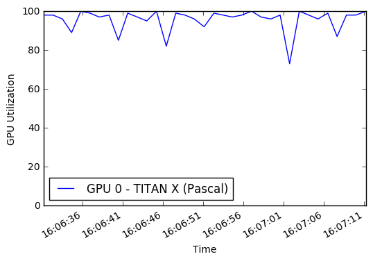
 % % time

# this is the augmentation configuration we will use for training
train_datagen = T . ImageDataGenerator (
    featurewise_center = False ,  # set input mean to 0 over the dataset
    samplewise_center = False ,  # set each sample mean to 0
    featurewise_std_normalization = False ,  # divide inputs by std of the dataset
    samplewise_std_normalization = False ,  # divide each input by its std
    zca_whitening = False ,  # apply ZCA whitening
    rotation_range = 0 ,  # randomly rotate images in the range (degrees, 0 to 180)
    width_shift_range = 0.2 ,  # randomly shift images horizontally (fraction of total width)
    height_shift_range = 0.2 ,  # randomly shift images vertically (fraction of total height)
    horizontal_flip = True ,  # randomly flip images
    vertical_flip = False , # randomly flip images
    zoom_range = [ .8 , 1 ],
    channel_shift_range = 30 ,
    fill_mode = 'reflect' )
train_datagen . config [ 'random_crop_size' ] = ( 299 , 299 )
train_datagen . set_pipeline ([ T . random_transform , T . random_crop , T . preprocess_input ])
train_generator = train_datagen . flow ( X_train , y_train_cat , batch_size = 64 , seed = 11 , pool = pool )
test_datagen = T . ImageDataGenerator ()
test_datagen . config [ 'random_crop_size' ] = ( 299 , 299 )
test_datagen . set_pipeline ([ T . random_transform , T . random_crop , T . preprocess_input ])
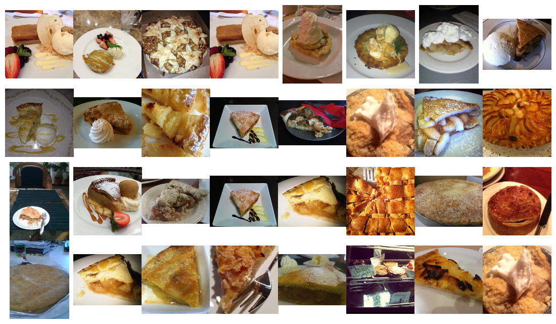
test_generator = test_datagen . flow ( X_test , y_test_cat , batch_size = 64 , seed = 11 , pool = pool )Мы видим, какие изображения выходят из этих идентификаторов:
 def reverse_preprocess_input ( x0 ):
    x = x0 / 2.0
    x += 0.5
    x *= 255.
    return x
% % time
@ interact ()
def show_images ( unprocess = True ):
for x in test_generator :
fig , axes = plt . subplots ( nrows = 8 , ncols = 4 )
fig . set_size_inches ( 8 , 8 )
page = 0
page_size = 32
start_i = page * page_size
for i , ax in enumerate ( axes . flat ):
img = x [ 0 ][ i + start_i ]
if unprocess :
im = ax . imshow ( reverse_preprocess_input ( img ). astype ( 'uint8' ) )
else :
im = ax . imshow ( img )
ax . set_axis_off ()
ax . title . set_visible ( False )
ax . xaxis . set_ticks ([])
ax . yaxis . set_ticks ([])
for spine in ax . spines . values ():
spine . set_visible ( False )
plt . subplots_adjust ( left = 0 , wspace = 0 , hspace = 0 )
plt . show ()
break 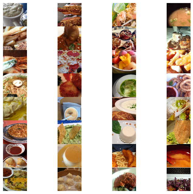
 CPU times: user 1.54 s, sys: 524 ms, total: 2.06 s
Wall time: 2.24 s
 % % time
show_images ( unprocess = False )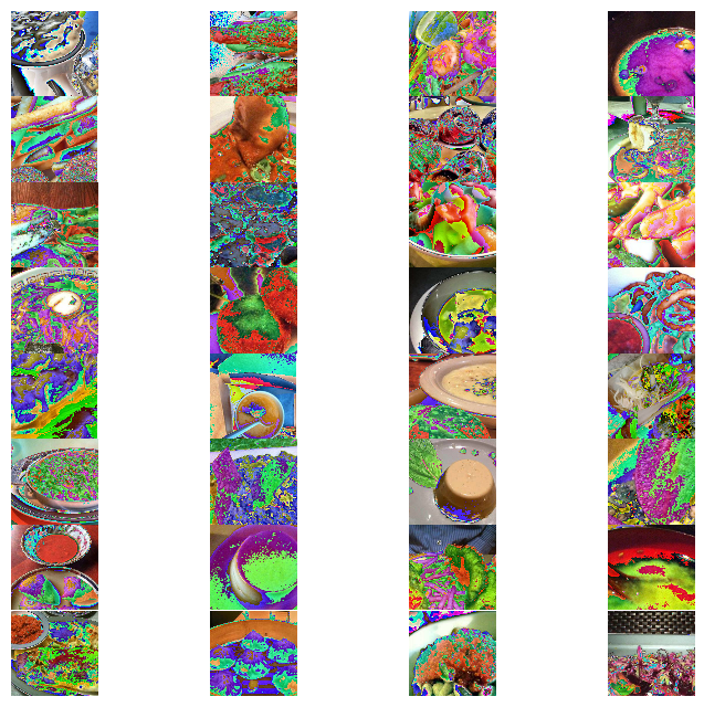
 CPU times: user 1.58 s, sys: 300 ms, total: 1.88 s
Wall time: 2.11 s
Мы будем переподтовать модель Google InceptionV3, предварительно подготовленную на ImageNet. Архитектура нейронной сети показана ниже.
 % % time
from keras . models import Sequential , Model
from keras . layers import Dense , Dropout , Activation , Flatten
from keras . layers import Convolution2D , MaxPooling2D , ZeroPadding2D , GlobalAveragePooling2D , AveragePooling2D
from keras . layers . normalization import BatchNormalization
from keras . preprocessing . image import ImageDataGenerator
from keras . callbacks import ModelCheckpoint , CSVLogger , LearningRateScheduler , ReduceLROnPlateau
from keras . optimizers import SGD
from keras . regularizers import l2
import keras . backend as K
import math

K . clear_session ()

base_model = InceptionV3 ( weights = 'imagenet' , include_top = False , input_tensor = Input ( shape = ( 299 , 299 , 3 )))
x = base_model . output
x = AveragePooling2D ( pool_size = ( 8 , 8 ))( x )
x = Dropout ( .4 )( x )
x = Flatten ()( x )
predictions = Dense ( n_classes , init = 'glorot_uniform' , W_regularizer = l2 ( .0005 ), activation = 'softmax' )( x )

model = Model ( input = base_model . input , output = predictions )

opt = SGD ( lr = .01 , momentum = .9 )
model . compile ( optimizer = opt , loss = 'categorical_crossentropy' , metrics = [ 'accuracy' ])

checkpointer = ModelCheckpoint ( filepath = 'model4.{epoch:02d}-{val_loss:.2f}.hdf5' , verbose = 1 , save_best_only = True )
csv_logger = CSVLogger ( 'model4.log' )

def schedule ( epoch ):
    if epoch < 15 :
        return .01
    elif epoch < 28 :
        return .002
    else :
        return .0004
lr_scheduler = LearningRateScheduler ( schedule )

model . fit_generator ( train_generator ,
                    validation_data = test_generator ,
                    nb_val_samples = X_test . shape [ 0 ],
                    samples_per_epoch = X_train . shape [ 0 ],
                    nb_epoch = 32 ,
                    verbose = 2 ,
                    callbacks = [ lr_scheduler , csv_logger , checkpointer ])
Epoch 1/32
Epoch 00000: val_loss improved from inf to 3.37355, saving model to model4.00-3.37.hdf5
1342s - loss: 4.2541 - acc: 0.0810 - val_loss: 3.3736 - val_acc: 0.2010
Epoch 2/32
Epoch 00001: val_loss improved from 3.37355 to 2.36625, saving model to model4.01-2.37.hdf5
1329s - loss: 2.9745 - acc: 0.3075 - val_loss: 2.3662 - val_acc: 0.4071
Epoch 3/32
Epoch 00002: val_loss improved from 2.36625 to 1.79355, saving model to model4.02-1.79.hdf5
1329s - loss: 2.3080 - acc: 0.4539 - val_loss: 1.7935 - val_acc: 0.5338
Epoch 4/32
Epoch 00003: val_loss improved from 1.79355 to 1.48898, saving model to model4.03-1.49.hdf5
1356s - loss: 2.0102 - acc: 0.5216 - val_loss: 1.4890 - val_acc: 0.6068
Epoch 5/32
Epoch 00004: val_loss improved from 1.48898 to 1.34121, saving model to model4.04-1.34.hdf5
1330s - loss: 1.8436 - acc: 0.5577 - val_loss: 1.3412 - val_acc: 0.6431
Epoch 6/32
Epoch 00005: val_loss improved from 1.34121 to 1.22485, saving model to model4.05-1.22.hdf5
1329s - loss: 1.7057 - acc: 0.5909 - val_loss: 1.2248 - val_acc: 0.6740
Epoch 7/32
Epoch 00006: val_loss did not improve
1328s - loss: 1.5996 - acc: 0.6126 - val_loss: 1.2310 - val_acc: 0.6716
Epoch 8/32
Epoch 00007: val_loss improved from 1.22485 to 1.11248, saving model to model4.07-1.11.hdf5
1331s - loss: 1.5148 - acc: 0.6314 - val_loss: 1.1125 - val_acc: 0.7022
Epoch 9/32
Epoch 00008: val_loss improved from 1.11248 to 1.07145, saving model to model4.08-1.07.hdf5
1331s - loss: 1.4395 - acc: 0.6506 - val_loss: 1.0714 - val_acc: 0.7095
Epoch 10/32
Epoch 00009: val_loss improved from 1.07145 to 1.05129, saving model to model4.09-1.05.hdf5
1333s - loss: 1.3900 - acc: 0.6637 - val_loss: 1.0513 - val_acc: 0.7181
Epoch 11/32
Epoch 00010: val_loss improved from 1.05129 to 1.03356, saving model to model4.10-1.03.hdf5
1331s - loss: 1.3316 - acc: 0.6780 - val_loss: 1.0336 - val_acc: 0.7250
Epoch 12/32
Epoch 00011: val_loss improved from 1.03356 to 1.00622, saving model to model4.11-1.01.hdf5
1331s - loss: 1.2850 - acc: 0.6893 - val_loss: 1.0062 - val_acc: 0.7275
Epoch 13/32
Epoch 00012: val_loss improved from 1.00622 to 0.94016, saving model to model4.12-0.94.hdf5
1330s - loss: 1.2325 - acc: 0.7003 - val_loss: 0.9402 - val_acc: 0.7461
Epoch 14/32
Epoch 00013: val_loss did not improve
1330s - loss: 1.1970 - acc: 0.7086 - val_loss: 0.9461 - val_acc: 0.7453
Epoch 15/32
Epoch 00014: val_loss did not improve
1329s - loss: 1.1683 - acc: 0.7154 - val_loss: 0.9691 - val_acc: 0.7396
Epoch 16/32
Epoch 00015: val_loss improved from 0.94016 to 0.71776, saving model to model4.15-0.72.hdf5
1329s - loss: 0.9398 - acc: 0.7724 - val_loss: 0.7178 - val_acc: 0.8055
Epoch 17/32
Epoch 00016: val_loss improved from 0.71776 to 0.70245, saving model to model4.16-0.70.hdf5
1329s - loss: 0.8591 - acc: 0.7916 - val_loss: 0.7025 - val_acc: 0.8069
Epoch 18/32
Epoch 00017: val_loss did not improve
1327s - loss: 0.8238 - acc: 0.8023 - val_loss: 0.7093 - val_acc: 0.8053
Epoch 19/32
Epoch 00018: val_loss did not improve
1327s - loss: 0.7947 - acc: 0.8093 - val_loss: 0.7048 - val_acc: 0.8059
Epoch 20/32
Epoch 00019: val_loss did not improve
1327s - loss: 0.7713 - acc: 0.8143 - val_loss: 0.7097 - val_acc: 0.8061
Epoch 21/32
Epoch 00020: val_loss improved from 0.70245 to 0.69545, saving model to model4.20-0.70.hdf5
1329s - loss: 0.7458 - acc: 0.8195 - val_loss: 0.6955 - val_acc: 0.8104
Epoch 22/32
Epoch 00021: val_loss did not improve
1328s - loss: 0.7282 - acc: 0.8232 - val_loss: 0.6977 - val_acc: 0.8119
Epoch 23/32
Epoch 00022: val_loss improved from 0.69545 to 0.69190, saving model to model4.22-0.69.hdf5
1328s - loss: 0.7114 - acc: 0.8284 - val_loss: 0.6919 - val_acc: 0.8150
Epoch 24/32
Epoch 00023: val_loss did not improve
1325s - loss: 0.6983 - acc: 0.8311 - val_loss: 0.7002 - val_acc: 0.8116
Epoch 25/32
Epoch 00024: val_loss did not improve
1330s - loss: 0.6719 - acc: 0.8381 - val_loss: 0.7031 - val_acc: 0.8112
Epoch 26/32
Epoch 00025: val_loss did not improve
1382s - loss: 0.6607 - acc: 0.8407 - val_loss: 0.7115 - val_acc: 0.8083
Epoch 27/32
Epoch 00026: val_loss did not improve
1330s - loss: 0.6479 - acc: 0.8439 - val_loss: 0.7037 - val_acc: 0.8126
Epoch 28/32
Epoch 00027: val_loss did not improve
1328s - loss: 0.6292 - acc: 0.8478 - val_loss: 0.7122 - val_acc: 0.8086
Epoch 29/32
Epoch 00028: val_loss improved from 0.69190 to 0.68908, saving model to model4.28-0.69.hdf5
1330s - loss: 0.5983 - acc: 0.8580 - val_loss: 0.6891 - val_acc: 0.8165
Epoch 30/32
Epoch 00029: val_loss improved from 0.68908 to 0.68740, saving model to model4.29-0.69.hdf5
1330s - loss: 0.5817 - acc: 0.8612 - val_loss: 0.6874 - val_acc: 0.8149
Epoch 31/32
Epoch 00030: val_loss did not improve
1328s - loss: 0.5729 - acc: 0.8642 - val_loss: 0.6912 - val_acc: 0.8143
Epoch 32/32
Epoch 00031: val_loss did not improve
1329s - loss: 0.5638 - acc: 0.8663 - val_loss: 0.6895 - val_acc: 0.8159
CPU times: user 8h 49min 20s, sys: 1h 55min 54s, total: 10h 45min 14s
Wall time: 11h 51min 18s
На этом этапе мы видим до 81,65 точность TOP-1 с одной урожаем в тестовом наборе. Мы можем продолжать обучать модель с еще более медленной скоростью обучения, чтобы увидеть, улучшится ли она больше.
В моих первоначальных экспериментах использовались более современные оптимизаторы, такие как Адам и Ададельта, наряду с более высокими показателями обучения. Я застрял на некоторое время ниже 80% точности, прежде чем решил более внимательно следовать литературе и использовать стохастический градиент спуск (SGD) с быстро уменьшающимся графиком обучения. Когда мы ищем многомерную поверхность, иногда иду медленнее, проходит долгий путь.
Из -за некоторой нестабильности с моим многопроцессорным кодом, иногда мне нужно перезапустить ноутбук, загрузить последнюю модель, а затем продолжить обучение.
 % % time
from keras . models import Sequential , Model , load_model
from keras . layers import Dense , Dropout , Activation , Flatten
from keras . layers import Convolution2D , MaxPooling2D , ZeroPadding2D , GlobalAveragePooling2D , AveragePooling2D
from keras . layers . normalization import BatchNormalization
from keras . preprocessing . image import ImageDataGenerator
from keras . callbacks import ModelCheckpoint , CSVLogger , LearningRateScheduler , ReduceLROnPlateau
from keras . optimizers import SGD
from keras . regularizers import l2
import keras . backend as K
import math

model = load_model ( filepath = './model4.29-0.69.hdf5' )

opt = SGD ( lr = .01 , momentum = .9 )
model . compile ( optimizer = opt , loss = 'categorical_crossentropy' , metrics = [ 'accuracy' ])

checkpointer = ModelCheckpoint ( filepath = 'model4b.{epoch:02d}-{val_loss:.2f}.hdf5' , verbose = 1 , save_best_only = True )
csv_logger = CSVLogger ( 'model4b.log' )

def schedule ( epoch ):
    if epoch < 10 :
        return .00008
    elif epoch < 20 :
        return .000016
    else :
        return .0000032

lr_scheduler = LearningRateScheduler ( schedule )

model . fit_generator ( train_generator ,
                    validation_data = test_generator ,
                    nb_val_samples = X_test . shape [ 0 ],
                    samples_per_epoch = X_train . shape [ 0 ],
                    nb_epoch = 32 ,
                    verbose = 2 ,
callbacks = [ lr_scheduler , csv_logger , checkpointer ]) На этом этапе у нас должно быть несколько обученных моделей, сохраненных на диск. Мы можем пройти через них и использовать функцию load_model для загрузки модели с самой низкой потерей / самой высокой точностью.
 % % time
#model = load_model(filepath='./model4.29-0.69.hdf5') # 86.8039 10-crop Top-1 test accuracy
model = load_model ( filepath = './model4b.10-0.68.hdf5' ) # 86.9703
CPU times: user 36.4 s, sys: 1.11 s, total: 37.5 s
Wall time: 36.5 s
Мы также хотим оценить тестовый набор с использованием нескольких сельскохозяйственных культур. Это может привести к повышению точности на 5% по сравнению с единственной оценкой урожая. Обычно использовать следующие культуры: верхний левый, верхний правый, нижний левый, внизу справа, в центре. Мы также принимаем те же культуры на изображении, перевернувшемся влево направо, создавая в общей сложности 10 культур.
Кроме того, мы хотим вернуть прогнозы Top-N для каждой культуры, например, чтобы рассчитать точность Top-5.
 def center_crop ( x , center_crop_size , ** kwargs ):
    centerw , centerh = x . shape [ 0 ] // 2 , x . shape [ 1 ] // 2
    halfw , halfh = center_crop_size [ 0 ] // 2 , center_crop_size [ 1 ] // 2
    return x [ centerw - halfw : centerw + halfw + 1 , centerh - halfh : centerh + halfh + 1 , :]
def predict_10_crop ( img , ix , top_n = 5 , plot = False , preprocess = True , debug = False ):
flipped_X = np . fliplr ( img )
crops = [
img [: 299 ,: 299 , :], # Upper Left
img [: 299 , img . shape [ 1 ] - 299 :, :], # Upper Right
img [ img . shape [ 0 ] - 299 :, : 299 , :], # Lower Left
img [ img . shape [ 0 ] - 299 :, img . shape [ 1 ] - 299 :, :], # Lower Right
center_crop ( img , ( 299 , 299 )),
flipped_X [: 299 ,: 299 , :],
flipped_X [: 299 , flipped_X . shape [ 1 ] - 299 :, :],
flipped_X [ flipped_X . shape [ 0 ] - 299 :, : 299 , :],
flipped_X [ flipped_X . shape [ 0 ] - 299 :, flipped_X . shape [ 1 ] - 299 :, :],
center_crop ( flipped_X , ( 299 , 299 ))
]
if preprocess :
crops = [ preprocess_input ( x . astype ( 'float32' )) for x in crops ]
if plot :
fig , ax = plt . subplots ( 2 , 5 , figsize = ( 10 , 4 ))
ax [ 0 ][ 0 ]. imshow ( crops [ 0 ])
ax [ 0 ][ 1 ]. imshow ( crops [ 1 ])
ax [ 0 ][ 2 ]. imshow ( crops [ 2 ])
ax [ 0 ][ 3 ]. imshow ( crops [ 3 ])
ax [ 0 ][ 4 ]. imshow ( crops [ 4 ])
ax [ 1 ][ 0 ]. imshow ( crops [ 5 ])
ax [ 1 ][ 1 ]. imshow ( crops [ 6 ])
ax [ 1 ][ 2 ]. imshow ( crops [ 7 ])
ax [ 1 ][ 3 ]. imshow ( crops [ 8 ])
ax [ 1 ][ 4 ]. imshow ( crops [ 9 ])
y_pred = model . predict ( np . array ( crops ))
preds = np . argmax ( y_pred , axis = 1 )
top_n_preds = np . argpartition ( y_pred , - top_n )[:, - top_n :]
if debug :
print ( 'Top-1 Predicted:' , preds )
print ( 'Top-5 Predicted:' , top_n_preds )
print ( 'True Label:' , y_test [ ix ])
return preds , top_n_preds
ix = 13001
predict_10_crop ( X_test [ ix ], ix , top_n = 5 , plot = True , preprocess = False , debug = True ) Top-1 Predicted: [74 74 74 74 74 74 74 74 74 74]
Top-5 Predicted: [[33 97 37 39 74]
[28 52 37 39 74]
[73 39 52 37 74]
[35 33 37 39 74]
[35 33 37 39 74]
[35 33 37 39 74]
[35 33 37 39 74]
[97 37 73 39 74]
[73 52 37 39 74]
[34 35 33 39 74]]
True Label: 88
(array([74, 74, 74, 74, 74, 74, 74, 74, 74, 74]), array([[33, 97, 37, 39, 74],
[28, 52, 37, 39, 74],
[73, 39, 52, 37, 74],
[35, 33, 37, 39, 74],
[35, 33, 37, 39, 74],
[35, 33, 37, 39, 74],
[35, 33, 37, 39, 74],
[97, 37, 73, 39, 74],
[73, 52, 37, 39, 74],
[34, 35, 33, 39, 74]]))
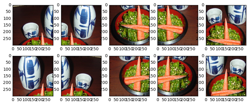
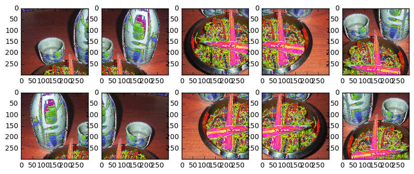
Нам также необходимо предварительно обработать изображения для модели на основе:
 ix = 13001
predict_10_crop ( X_test [ ix ], ix , top_n = 5 , plot = True , preprocess = True , debug = True )
Top-1 Predicted: [51 51 88 88 88 51 51 88 88 88]
Top-5 Predicted: [[18 79 51 13 48]
[48 79 11 55 51]
[79 93 81 37 88]
[51 86 93 81 88]
[11 79 51 81 88]
[19 79 51 56 13]
[11 88 48 51 13]
[37 93 86 88 81]
[37 79 93 88 81]
[84 81 11 79 88]]
True Label: 88
(array([51, 51, 88, 88, 88, 51, 51, 88, 88, 88]), array([[18, 79, 51, 13, 48],
[48, 79, 11, 55, 51],
[79, 93, 81, 37, 88],
[51, 86, 93, 81, 88],
[11, 79, 51, 81, 88],
[19, 79, 51, 56, 13],
[11, 88, 48, 51, 13],
[37, 93, 86, 88, 81],
[37, 79, 93, 88, 81],
[84, 81, 11, 79, 88]]))
Теперь мы создаем культуры для каждого элемента в тестовом наборе и получаем прогнозы. В настоящее время это медленный процесс, так как я не пользуюсь многопроцессоровкой или другими типами параллелизма.
 % % time
preds_10_crop = {}
for ix in range ( len ( X_test )):
    if ix % 1000 == 0 :
        print ( ix )
    preds_10_crop [ ix ] = predict_10_crop ( X_test [ ix ], ix )
0
1000
2000
3000
4000
5000
6000
7000
8000
9000
10000
11000
12000
13000
14000
15000
16000
17000
18000
19000
20000
21000
22000
23000
24000
25000
CPU times: user 50min 3s, sys: 5min 13s, total: 55min 16s
Wall time: 31min 28s
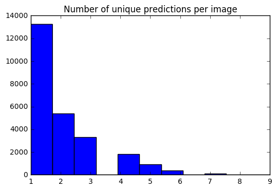
Теперь у нас есть набор из 10 прогнозов для каждого изображения. Используя гистограмму, я могу увидеть, как распространяется # уникальных прогнозов для каждого изображения.
 preds_uniq = { k : np . unique ( v [ 0 ]) for k , v in preds_10_crop . items ()}
preds_hist = np . array ([ len ( x ) for x in preds_uniq . values ()])

plt . hist ( preds_hist , bins = 11 )
plt . title ( 'Number of unique predictions per image' )
<matplotlib.text.Text at 0x7fe30c3daa20>
Давайте создадим словарь, чтобы отобразить индекс тестового элемента с предсказаниями TOP-1 / TOP-5.
 preds_top_1 = { k : collections . Counter ( v [ 0 ]). most_common ( 1 ) for k , v in preds_10_crop . items ()}

top_5_per_ix = { k : collections . Counter ( preds_10_crop [ k ][ 1 ]. reshape ( - 1 )). most_common ( 5 )
                for k , v in preds_10_crop . items ()}
preds_top_5 = { k : [ y [ 0 ] for y in v ] for k , v in top_5_per_ix . items ()}
% % time
right_counter = 0
for i in range ( len ( y_test )):
guess , actual = preds_top_1 [ i ][ 0 ][ 0 ], y_test [ i ]
if guess == actual :
right_counter += 1
print ( 'Top-1 Accuracy, 10-Crop: {0:.2f}%' . format ( right_counter / len ( y_test ) * 100 )) Top-1 Accuracy, 10-Crop: 86.97%
CPU times: user 28 ms, sys: 0 ns, total: 28 ms
Wall time: 27.3 ms
 % % time
top_5_counter = 0
for i in range ( len ( y_test )):
    guesses , actual = preds_top_5 [ i ], y_test [ i ]
    if actual in guesses :
        top_5_counter += 1

print ( 'Top-5 Accuracy, 10-Crop: {0:.2f}%' . format ( top_5_counter / len ( y_test ) * 100 ))
Top-5 Accuracy, 10-Crop: 97.42%
CPU times: user 28 ms, sys: 0 ns, total: 28 ms
Wall time: 27 ms
y_pred = [ x [ 0 ][ 0 ] for x in preds_top_1 . values ()] @ interact ( page = [ 0 , int ( len ( X_test ) / 20 )])
def show_images_prediction ( page = 0 ):
page_size = 20
nrows = 4
ncols = 5
fig , axes = plt . subplots ( nrows = nrows , ncols = ncols , figsize = ( 12 , 12 ))
fig . set_size_inches ( 12 , 8 )
#fig.tight_layout()
#imgs = np.random.choice((y_all == n_class).nonzero()[0], nrows * ncols)
start_i = page * page_size
for i , ax in enumerate ( axes . flat ):
im = ax . imshow ( X_test [ i + start_i ])
ax . set_axis_off ()
ax . title . set_visible ( False )
ax . xaxis . set_ticks ([])
ax . yaxis . set_ticks ([])
for spine in ax . spines . values ():
spine . set_visible ( False )
predicted = ix_to_class [ y_pred [ i + start_i ]]
match = predicted == ix_to_class [ y_test [ start_i + i ]]
ec = ( 1 , .5 , .5 )
fc = ( 1 , .8 , .8 )
if match :
ec = ( 0 , .6 , .1 )
fc = ( 0 , .7 , .2 )
# predicted label
ax . text ( 0 , 400 , 'P: ' + predicted , size = 10 , rotation = 0 ,
ha = "left" , va = "top" ,
bbox = dict ( boxstyle = "round" ,
ec = ec ,
fc = fc ,
)
)
if not match :
# true label
ax . text ( 0 , 480 , 'A: ' + ix_to_class [ y_test [ start_i + i ]], size = 10 , rotation = 0 ,
ha = "left" , va = "top" ,
bbox = dict ( boxstyle = "round" ,
ec = ec ,
fc = fc ,
)
)
plt . subplots_adjust ( left = 0 , wspace = 1 , hspace = 0 )
plt . show ()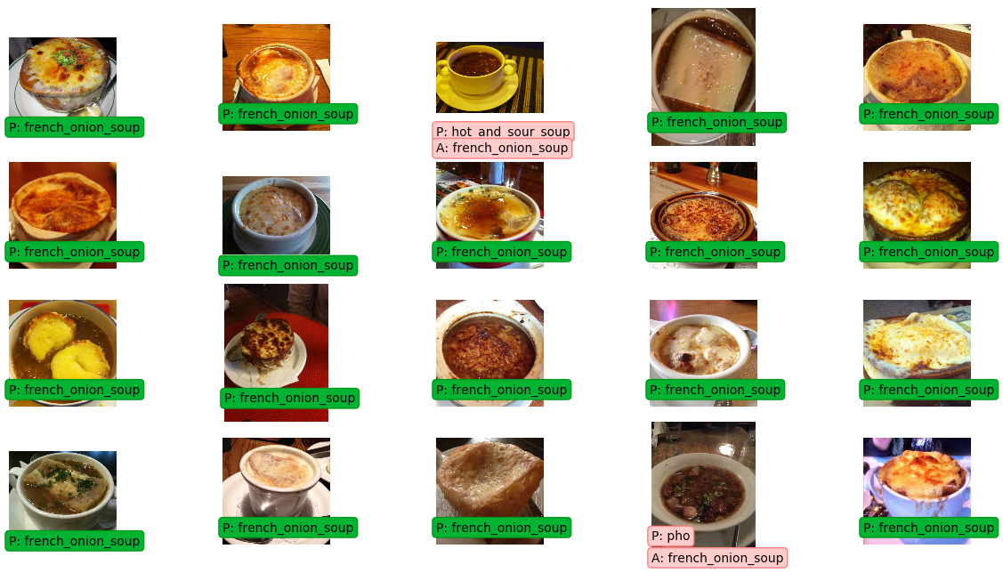
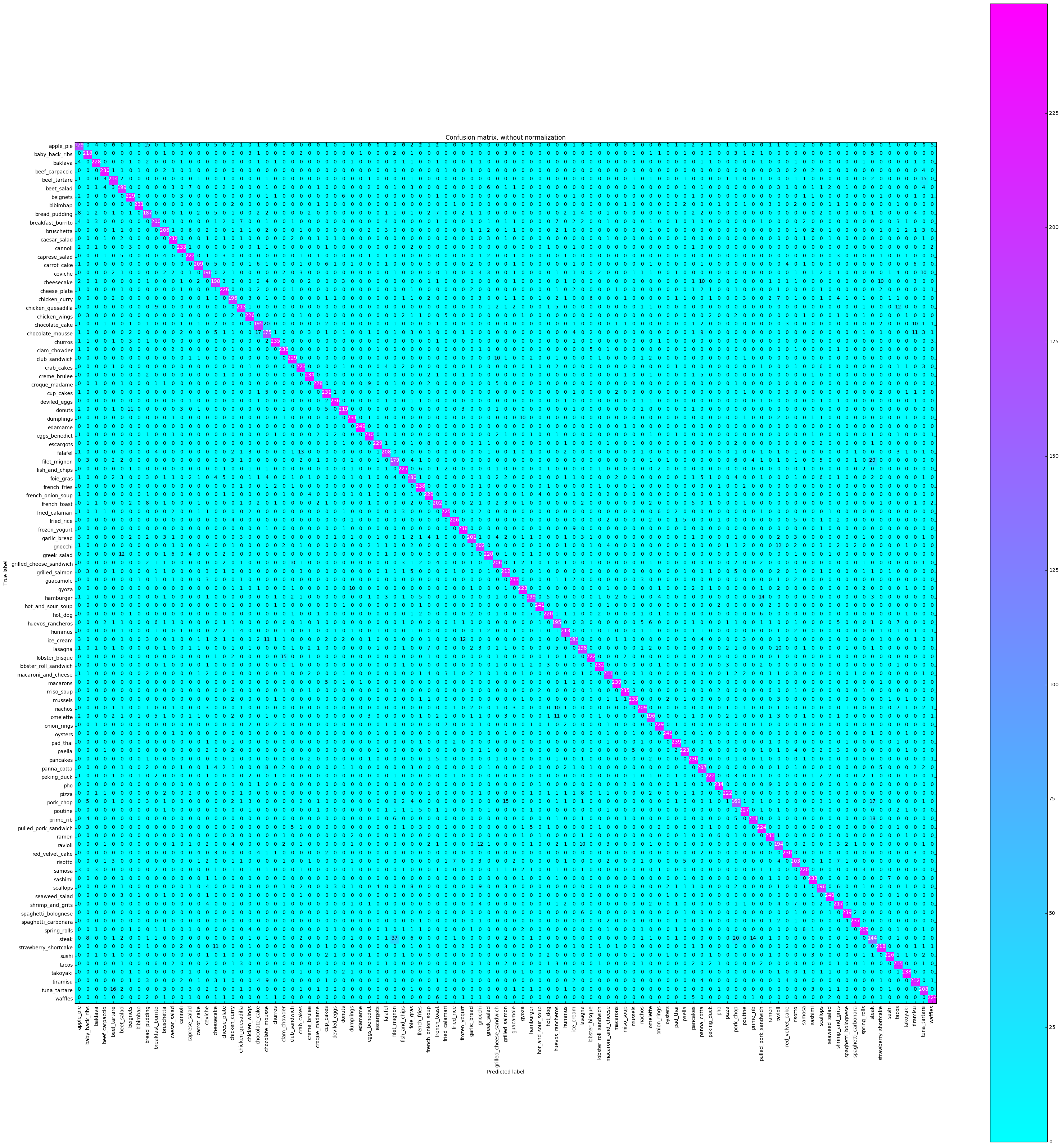
Матрица путаницы будет построить каждую метку класса, и сколько раз она была правильно помечена по сравнению с другим раз, она была неправильно помечена как другой класс.
 % % time
from sklearn . metrics import confusion_matrix
import itertools

def plot_confusion_matrix ( cm , classes ,
                          normalize = False ,
                          title = 'Confusion matrix' ,
                          cmap = plt . cm . Blues ):
    """
    This function prints and plots the confusion matrix.
    Normalization can be applied by setting `normalize=True`.
    """
    plt . imshow ( cm , interpolation = 'nearest' , cmap = cmap )
    plt . title ( title )
    plt . colorbar ()
    tick_marks = np . arange ( len ( classes ))
    plt . xticks ( tick_marks , classes , rotation = 90 )
    plt . yticks ( tick_marks , classes )

    if normalize :
        cm = cm . astype ( 'float' ) / cm . sum ( axis = 1 )[:, np . newaxis ]
        print ( "Normalized confusion matrix" )
    else :
        print ( 'Confusion matrix, without normalization' )

    print ( cm )

    thresh = cm . max () / 2.
    for i , j in itertools . product ( range ( cm . shape [ 0 ]), range ( cm . shape [ 1 ])):
        plt . text ( j , i , cm [ i , j ],
                 horizontalalignment = "center" ,
                 color = "white" if cm [ i , j ] > thresh else "black" )

    plt . tight_layout ()
    plt . ylabel ( 'True label' )
    plt . xlabel ( 'Predicted label' )


# Compute confusion matrix
cnf_matrix = confusion_matrix ( y_test , y_pred )
np . set_printoptions ( precision = 2 )

class_names = [ ix_to_class [ i ] for i in range ( 101 )]

plt . figure ()
fig = plt . gcf ()
fig . set_size_inches ( 32 , 32 )
plot_confusion_matrix ( cnf_matrix , classes = class_names ,
                      title = 'Confusion matrix, without normalization' ,
                      cmap = plt . cm . cool )
plt . show ()
Confusion matrix, without normalization
[[179 0 4 ..., 2 0 5]
[ 0 218 0 ..., 0 0 0]
[ 4 0 228 ..., 1 0 0]
...,
[ 0 0 0 ..., 212 0 1]
[ 0 0 0 ..., 0 208 0]
[ 0 0 0 ..., 0 0 224]]
 CPU times: user 16.4 s, sys: 1.22 s, total: 17.6 s
Wall time: 16.4 s
Мы хотим посмотреть, была ли точность последовательной во всех классах, или некоторые классы были намного проще / труднее пометить, чем другие. Согласно нашему заговору, несколько классов были выбросами с точки зрения того, что их гораздо сложнее назвать правильно.
 corrects = collections . defaultdict ( int )
incorrects = collections . defaultdict ( int )
for ( pred , actual ) in zip ( y_pred , y_test ):
    if pred == actual :
        corrects [ actual ] += 1
    else :
        incorrects [ actual ] += 1

class_accuracies = {}
for ix in range ( 101 ):
    class_accuracies [ ix ] = corrects [ ix ] / 250

plt . hist ( list ( class_accuracies . values ()), bins = 20 )
plt . title ( 'Accuracy by Class histogram' )
<matplotlib.text.Text at 0x7fe2d5d4f860>
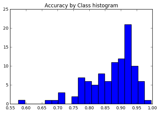
 sorted_class_accuracies = sorted ( class_accuracies . items (), key = lambda x : - x [ 1 ])
[( ix_to_class [ c [ 0 ]], c [ 1 ]) for c in sorted_class_accuracies ]
[('edamame', 0.996),
('hot_and_sour_soup', 0.964),
('oysters', 0.964),
('seaweed_salad', 0.96),
('macarons', 0.956),
('pad_thai', 0.956),
('spaghetti_bolognese', 0.956),
('french_fries', 0.952),
('frozen_yogurt', 0.952),
('takoyaki', 0.952),
('spaghetti_carbonara', 0.948),
('clam_chowder', 0.944),
('deviled_eggs', 0.944),
('churros', 0.94),
('miso_soup', 0.94),
('creme_brulee', 0.936),
('pho', 0.936),
('cannoli', 0.932),
('guacamole', 0.932),
('mussels', 0.932),
('sashimi', 0.932),
('caesar_salad', 0.928),
('lobster_roll_sandwich', 0.928),
('bibimbap', 0.924),
('cup_cakes', 0.924),
('dumplings', 0.924),
('ramen', 0.924),
('beef_carpaccio', 0.92),
('eggs_benedict', 0.92),
('pancakes', 0.92),
('red_velvet_cake', 0.92),
('beignets', 0.916),
('club_sandwich', 0.916),
('escargots', 0.916),
('french_onion_soup', 0.916),
('onion_rings', 0.916),
('baklava', 0.912),
('croque_madame', 0.912),
('fish_and_chips', 0.908),
('poutine', 0.908),
('cheese_plate', 0.904),
('chicken_wings', 0.904),
('fried_rice', 0.904),
('sushi', 0.904),
('fried_calamari', 0.9),
('pulled_pork_sandwich', 0.896),
('waffles', 0.896),
('crab_cakes', 0.892),
('gyoza', 0.892),
('paella', 0.892),
('caprese_salad', 0.888),
('lobster_bisque', 0.888),
('peking_duck', 0.888),
('pizza', 0.888),
('greek_salad', 0.88),
('hot_dog', 0.88),
('samosa', 0.88),
('donuts', 0.876),
('spring_rolls', 0.876),
('baby_back_ribs', 0.872),
('strawberry_shortcake', 0.872),
('shrimp_and_grits', 0.868),
('tacos', 0.86),
('beef_tartare', 0.856),
('prime_rib', 0.856),
('chicken_quesadilla', 0.852),
('hummus', 0.852),
('grilled_salmon', 0.848),
('tiramisu', 0.848),
('macaroni_and_cheese', 0.844),
('carrot_cake', 0.836),
('nachos', 0.836),
('falafel', 0.832),
('tuna_tartare', 0.832),
('panna_cotta', 0.828),
('bruschetta', 0.824),
('grilled_cheese_sandwich', 0.824),
('risotto', 0.812),
('french_toast', 0.808),
('gnocchi', 0.808),
('garlic_bread', 0.804),
('breakfast_burrito', 0.8),
('beet_salad', 0.796),
('hamburger', 0.796),
('cheesecake', 0.792),
('lasagna', 0.792),
('ceviche', 0.784),
('chicken_curry', 0.784),
('omelette', 0.784),
('scallops', 0.784),
('chocolate_cake', 0.78),
('huevos_rancheros', 0.78),
('ravioli', 0.776),
('ice_cream', 0.764),
('bread_pudding', 0.748),
('foie_gras', 0.72),
('apple_pie', 0.716),
('filet_mignon', 0.716),
('chocolate_mousse', 0.7),
('pork_chop', 0.676),
('steak', 0.576)]
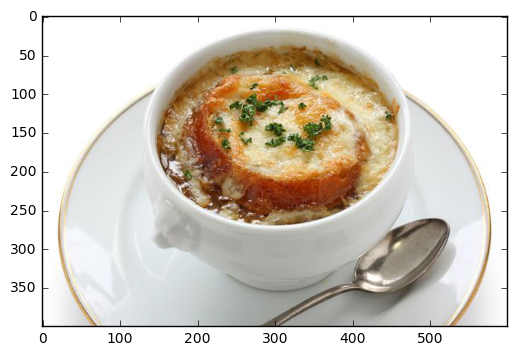
Прогноз из локального файла
 pic_path = '/home/stratospark/Downloads/soup.jpg'
pic = img . imread ( pic_path )
preds = predict_10_crop ( np . array ( pic ), 0 )[ 0 ]
best_pred = collections . Counter ( preds ). most_common ( 1 )[ 0 ][ 0 ]
print ( ix_to_class [ best_pred ])
plt . imshow ( pic )
french_onion_soup
<matplotlib.image.AxesImage at 0x7fe2d59eb5c0>
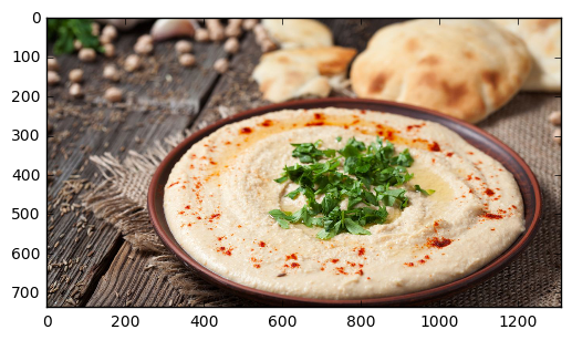
Прогнозирование с изображения в Интернете
 import urllib . request

@ interact
def predict_remote_image ( url = 'http://themodelhouse.tv/wp-content/uploads/2016/08/hummus.jpg' ):
    with urllib . request . urlopen ( url ) as f :
        pic = plt . imread ( f , format = 'jpg' )
        preds = predict_10_crop ( np . array ( pic ), 0 )[ 0 ]
        best_pred = collections . Counter ( preds ). most_common ( 1 )[ 0 ][ 0 ]
        print ( ix_to_class [ best_pred ])
        plt . imshow ( pic )
hummus
 with open ( 'model.json' , 'w' ) as f :
    f . write ( model . to_json ())
import json
json . dumps ( ix_to_class ) '{"0": "apple_pie", "1": "baby_back_ribs", "2": "baklava", "3": "beef_carpaccio", "4": "beef_tartare", "5": "beet_salad", "6": "beignets", "7": "bibimbap", "8": "bread_pudding", "9": "breakfast_burrito", "10": "bruschetta", "11": "caesar_salad", "12": "cannoli", "13": "caprese_salad", "14": "carrot_cake", "15": "ceviche", "16": "cheesecake", "17": "cheese_plate", "18": "chicken_curry", "19": "chicken_quesadilla", "20": "chicken_wings", "21": "chocolate_cake", "22": "chocolate_mousse", "23": "churros", "24": "clam_chowder", "25": "club_sandwich", "26": "crab_cakes", "27": "creme_brulee", "28": "croque_madame", "29": "cup_cakes", "30": "deviled_eggs", "31": "donuts", "32": "dumplings", "33": "edamame", "34": "eggs_benedict", "35": "escargots", "36": "falafel", "37": "filet_mignon", "38": "fish_and_chips", "39": "foie_gras", "40": "french_fries", "41": "french_onion_soup", "42": "french_toast", "43": "fried_calamari", "44": "fried_rice", "45": "frozen_yogurt", "46": "garlic_bread", "47": "gnocchi", "48": "greek_salad", "49": "grilled_cheese_sandwich", "50": "grilled_salmon", "51": "guacamole", "52": "gyoza", "53": "hamburger", "54": "hot_and_sour_soup", "55": "hot_dog", "56": "huevos_rancheros", "57": "hummus", "58": "ice_cream", "59": "lasagna", "60": "lobster_bisque", "61": "lobster_roll_sandwich", "62": "macaroni_and_cheese", "63": "macarons", "64": "miso_soup", "65": "mussels", "66": "nachos", "67": "omelette", "68": "onion_rings", "69": "oysters", "70": "pad_thai", "71": "paella", "72": "pancakes", "73": "panna_cotta", "74": "peking_duck", "75": "pho", "76": "pizza", "77": "pork_chop", "78": "poutine", "79": "prime_rib", "80": "pulled_pork_sandwich", "81": "ramen", "82": "ravioli", "83": "red_velvet_cake", "84": "risotto", "85": "samosa", "86": "sashimi", "87": "scallops", "88": "seaweed_salad", "89": "shrimp_and_grits", "90": "spaghetti_bolognese", "91": "spaghetti_carbonara", "92": "spring_rolls", "93": "steak", "94": "strawberry_shortcake", "95": "sushi", "96": "tacos", "97": "takoyaki", "98": "tiramisu", "99": "tuna_tartare", "100": "waffles"}'


