food 101 keras
1.0.0
 from IPython . display import HTML , Image

url = 'http://stratospark.com/demos/food-101/'
el = '<' + 'iframe src="{}"' . format ( url ) + ' width="100%" height=600></iframe>' # prevent notebook render bug
HTML ( el )Github에서 이것을 읽고 있다면 데모는 다음과 같습니다. 내 블로그에서 라이브 데모를 보려면 아래 링크를 따르십시오.
Image ( 'demo.jpg' )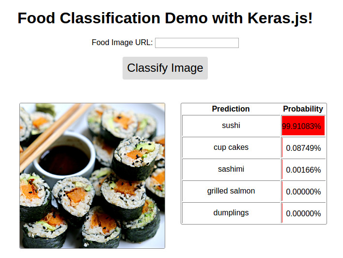
@ http://blog.stratospark.com/deep-learning-applied-classification-learning-keras.html 사용 가능합니다
@ https://github.com/stratospark/food-101-keras 사용 가능
업데이트
더 넓은 딥 러닝 분야의 기술인 CNN (Convolutional Neural Networks)은 컴퓨터 비전 응용 분야의 혁신적인 힘, 특히 과거의 반쯤 정도. 주요 사용 사례 중 하나는 이미지 분류의 것입니다. 예를 들어 그림이 개 또는 고양이의 그림인지 여부를 결정합니다.
물론 이진 분류기로 자신을 제한 할 필요는 없습니다. CNN은 컴퓨터 비전 알고리즘 성능을 벤치마킹하는 데 사용되는 1000 개의 클래스의 잘 알려진 Imagenet 데이터 세트에서 볼 수 있듯이 수천 개의 다른 클래스로 쉽게 확장 할 수 있습니다.
지난 몇 년 동안, 이러한 최첨단 기술은 광범위한 소프트웨어 개발 커뮤니티에서 이용할 수있게되기 시작했습니다. TensorFlow와 같은 산업 강도 패키지는 GPU 매트릭스 작업, 부분 미분 기울기 및 확률 적 최적화기를 핸드 코딩하지 않고도 클라우드의 확장 가능한 클러스터에 임베디드/모바일 장치를 위해 딥 러닝 애플리케이션을 작성하는 데 사용하는 것과 동일한 빌딩 블록을 제공했습니다. 효율적인 응용 프로그램을 가능하게합니다.
무엇보다도, Keras와 같은 사용자 친화적 인 API는 더 낮은 수준 세부 사항 중 일부를 추상화하고 딥 러닝 계산 그래프를 빠르게 프로토 타이핑하는 데 집중할 수 있도록합니다. 우리가 레고를 혼합하고 일치시키기 위해 원하는 결과를 얻는 것과 마찬가지로.
나 자신을위한 소개 프로젝트로서, 나는 Keras와 함께 제공되는 미리 훈련 된 이미지 분류기를 사용하고 흥미로운 데이터 세트에서 재교육을 선택했습니다. 나는 좋은 음식과 가정 요리에 매우 많이 들어가서 그 선을 따라 무언가가 식욕을 돋우고있었습니다.
이 논문에서 Food-101-임의의 숲을 가진 차별적 구성 요소를 채굴하여 Food-101 데이터 세트를 소개합니다. 101 개의 다양한 종류의 음식이 있으며, 감독 훈련을 위해 수업 당 1000 개의 레이블이 붙은 이미지가 있습니다.
이 Keras 블로그 게시물에서 영감을 얻었습니다. 데이터가 거의없는 강력한 이미지 분류 모델 구축과 Github에서 찾은 관련 스크립트 : Keras-Finetuning.
나는 최근에 딥 러닝을 실험 할 목적으로 시스템을 구축했습니다. 주요 구성 요소는 12GB의 메모리가있는 Nvidia Titan X Pascal, 96GB 시스템 RAM 및 12 코어 인텔 코어 i7입니다. 64 비트 Ubuntu 16.04를 실행하고 Anaconda Python 분포를 사용하고 있습니다. 불행히도, 당신은 RAM이 충분하지 않으면 자신의 시스템 에서이 노트북을 따라갈 수 없습니다. 앞으로는 RAM보다 더 크게 처리하는 방법을 배우고 싶습니다. 아이디어가 있으면 연락하십시오!
나는 약 1 개월 동안이 프로젝트를 구축하고 수십 개의 모델을 훈련시키고 더 빠른 이미지 확대를 위해 멀티 프로세싱과 같은 다양한 영역을 탐색하려고 노력했습니다. 이것은 2017 년 1 월 22 일 기준으로 최고의 성과를내는 모델을 포함하는 노트북의 정리 버전입니다.
사전 훈련 된 Google InceptionV3 모델을 미세 조정 한 후 항목 당 단일 작물을 사용하여 테스트 세트에서 약 82.03% 상위 1 위 정확도를 달성 할 수있었습니다. 예제 당 10 개의 작물을 사용하고 가장 빈번한 예측 클래스 (ES)를 사용하여 86.97% 상위 1 위 정확도 와 97.42% 상위 정확도를 달성 할 수있었습니다.
다른 사람들은보다 정확한 결과를 얻을 수있었습니다.
구현! 확인 : http://blog.stratospark.com/creating-a-deep-learning-ios-app-with-keras-and-tensorflow.html
노트북의 나머지 부분에 필요한 모든 패키지를 가져 오겠습니다.
 import matplotlib . pyplot as plt
import matplotlib . image as img
import numpy as np
from scipy . misc import imresize

% matplotlib inline

import os
from os import listdir
from os . path import isfile , join
import shutil
import stat
import collections
from collections import defaultdict

from ipywidgets import interact , interactive , fixed
import ipywidgets as widgets

import h5py
from sklearn . model_selection import train_test_split
from keras . utils . np_utils import to_categorical
from keras . applications . inception_v3 import preprocess_input
from keras . models import load_model
Using TensorFlow backend.
데이터 세트를 다운로드하여 노트북 폴더 내에서 추출하십시오. 별도의 터미널 창 에서이 작업을 수행하는 것이 더 쉬울 수 있습니다.
# !wget http://data.vision.ee.ethz.ch/cvl/food-101.tar.gz # !tar xzvf food-101.tar.gz여기에 어떤 종류의 음식이 표시되는지 봅시다.
!l s food - 101 / images apple_pie eggs_benedict onion_rings
baby_back_ribs escargots oysters
baklava falafel pad_thai
beef_carpaccio filet_mignon paella
beef_tartare fish_and_chips pancakes
beet_salad foie_gras panna_cotta
beignets french_fries peking_duck
bibimbap french_onion_soup pho
bread_pudding french_toast pizza
breakfast_burrito fried_calamari pork_chop
bruschetta fried_rice poutine
caesar_salad frozen_yogurt prime_rib
cannoli garlic_bread pulled_pork_sandwich
caprese_salad gnocchi ramen
carrot_cake greek_salad ravioli
ceviche grilled_cheese_sandwich red_velvet_cake
cheesecake grilled_salmon risotto
cheese_plate guacamole samosa
chicken_curry gyoza sashimi
chicken_quesadilla hamburger scallops
chicken_wings hot_and_sour_soup seaweed_salad
chocolate_cake hot_dog shrimp_and_grits
chocolate_mousse huevos_rancheros spaghetti_bolognese
churros hummus spaghetti_carbonara
clam_chowder ice_cream spring_rolls
club_sandwich lasagna steak
crab_cakes lobster_bisque strawberry_shortcake
creme_brulee lobster_roll_sandwich sushi
croque_madame macaroni_and_cheese tacos
cup_cakes macarons takoyaki
deviled_eggs miso_soup tiramisu
donuts mussels tuna_tartare
dumplings nachos waffles
edamame omelette
!l s food - 101 / images / apple_pie / | head - 10 1005649.jpg
1011328.jpg
101251.jpg
1014775.jpg
1026328.jpg
1028787.jpg
1034399.jpg
103801.jpg
1038694.jpg
1043283.jpg
ls: write error: Broken pipe
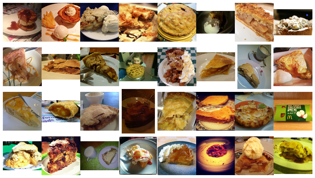
각 음식 수업의 임의의 이미지를 살펴 보겠습니다. 새 창에서 이미지를 마우스 오른쪽 버튼으로 클릭하고 열거나 저장하여 더 높은 해상도로 볼 수 있습니다.
 root_dir = 'food-101/images/'
rows = 17
cols = 6
fig , ax = plt . subplots ( rows , cols , frameon = False , figsize = ( 15 , 25 ))
fig . suptitle ( 'Random Image from Each Food Class' , fontsize = 20 )
sorted_food_dirs = sorted ( os . listdir ( root_dir ))
for i in range ( rows ):
    for j in range ( cols ):
        try :
            food_dir = sorted_food_dirs [ i * cols + j ]
        except :
            break
        all_files = os . listdir ( os . path . join ( root_dir , food_dir ))
        rand_img = np . random . choice ( all_files )
        img = plt . imread ( os . path . join ( root_dir , food_dir , rand_img ))
        ax [ i ][ j ]. imshow ( img )
        ec = ( 0 , .6 , .1 )
        fc = ( 0 , .7 , .2 )
        ax [ i ][ j ]. text ( 0 , - 20 , food_dir , size = 10 , rotation = 0 ,
                ha = "left" , va = "top" ,
                bbox = dict ( boxstyle = "round" , ec = ec , fc = fc ))
plt . setp ( ax , xticks = [], yticks = [])
plt . tight_layout ( rect = [ 0 , 0.03 , 1 , 0.95 ])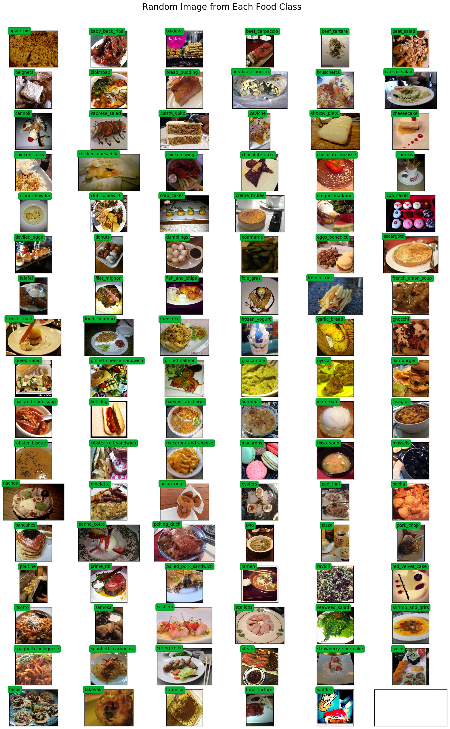
multiprocessing.Pool .pool은 훈련 중 이미지 확대를 가속화하는 데 사용됩니다.
 # Setup multiprocessing pool
# Do this early, as once images are loaded into memory there will be Errno 12
# http://stackoverflow.com/questions/14749897/python-multiprocessing-memory-usage
import multiprocessing as mp

num_processes = 6
pool = mp . Pool ( processes = num_processes )
적절한 라벨 인코딩 및 예쁜 인쇄를 위해 클래스에서 색인까지의지도가 필요합니다.
 class_to_ix = {}
ix_to_class = {}
with open ( 'food-101/meta/classes.txt' , 'r' ) as txt :
    classes = [ l . strip () for l in txt . readlines ()]
    class_to_ix = dict ( zip ( classes , range ( len ( classes ))))
    ix_to_class = dict ( zip ( range ( len ( classes )), classes ))
    class_to_ix = { v : k for k , v in ix_to_class . items ()}
sorted_class_to_ix = collections . OrderedDict ( sorted ( class_to_ix . items ()))
Food-101 데이터 세트에는 제공된 열차/테스트 분할이 있습니다. 분류 성능을 다른 구현과 비교하기 위해 이것을 사용하려고합니다.
 # Only split files if haven't already
if not os . path . isdir ( './food-101/test' ) and not os . path . isdir ( './food-101/train' ):

    def copytree ( src , dst , symlinks = False , ignore = None ):
        if not os . path . exists ( dst ):
            os . makedirs ( dst )
            shutil . copystat ( src , dst )
        lst = os . listdir ( src )
        if ignore :
            excl = ignore ( src , lst )
            lst = [ x for x in lst if x not in excl ]
        for item in lst :
            s = os . path . join ( src , item )
            d = os . path . join ( dst , item )
            if symlinks and os . path . islink ( s ):
                if os . path . lexists ( d ):
                    os . remove ( d )
                os . symlink ( os . readlink ( s ), d )
                try :
                    st = os . lstat ( s )
                    mode = stat . S_IMODE ( st . st_mode )
                    os . lchmod ( d , mode )
                except :
                    pass # lchmod not available
            elif os . path . isdir ( s ):
                copytree ( s , d , symlinks , ignore )
            else :
                shutil . copy2 ( s , d )

    def generate_dir_file_map ( path ):
        dir_files = defaultdict ( list )
        with open ( path , 'r' ) as txt :
            files = [ l . strip () for l in txt . readlines ()]
            for f in files :
                dir_name , id = f . split ( '/' )
                dir_files [ dir_name ]. append ( id + '.jpg' )
        return dir_files

    train_dir_files = generate_dir_file_map ( 'food-101/meta/train.txt' )
    test_dir_files = generate_dir_file_map ( 'food-101/meta/test.txt' )


    def ignore_train ( d , filenames ):
        print ( d )
        subdir = d . split ( '/' )[ - 1 ]
        to_ignore = train_dir_files [ subdir ]
        return to_ignore

    def ignore_test ( d , filenames ):
        print ( d )
        subdir = d . split ( '/' )[ - 1 ]
        to_ignore = test_dir_files [ subdir ]
        return to_ignore

    copytree ( 'food-101/images' , 'food-101/test' , ignore = ignore_train )
    copytree ( 'food-101/images' , 'food-101/train' , ignore = ignore_test )

else :
    print ( 'Train/Test files already copied into separate folders.' )
Train/Test files already copied into separate folders.
이제 우리는 훈련 및 테스트 이미지를 메모리에로드 할 준비가되었습니다. 모든 것이로드되면 약 80GB의 메모리가 할당됩니다.
min_size 보다 너비 또는 길이가 작은 이미지는 크기가 조정됩니다. 이것은 이미지 확대 중에 적절한 크기의 작물을 섭취 할 수 있도록하기 위해서입니다.
 % % time

# Load dataset images and resize to meet minimum width and height pixel size
def load_images ( root , min_side = 299 ):
    all_imgs = []
    all_classes = []
    resize_count = 0
    invalid_count = 0
    for i , subdir in enumerate ( listdir ( root )):
        imgs = listdir ( join ( root , subdir ))
        class_ix = class_to_ix [ subdir ]
        print ( i , class_ix , subdir )
        for img_name in imgs :
            img_arr = img . imread ( join ( root , subdir , img_name ))
            img_arr_rs = img_arr
            try :
                w , h , _ = img_arr . shape
                if w < min_side :
                    wpercent = ( min_side / float ( w ))
                    hsize = int (( float ( h ) * float ( wpercent )))
                    #print('new dims:', min_side, hsize)
                    img_arr_rs = imresize ( img_arr , ( min_side , hsize ))
                    resize_count += 1
                elif h < min_side :
                    hpercent = ( min_side / float ( h ))
                    wsize = int (( float ( w ) * float ( hpercent )))
                    #print('new dims:', wsize, min_side)
                    img_arr_rs = imresize ( img_arr , ( wsize , min_side ))
                    resize_count += 1
                all_imgs . append ( img_arr_rs )
                all_classes . append ( class_ix )
            except :
                print ( 'Skipping bad image: ' , subdir , img_name )
                invalid_count += 1
    print ( len ( all_imgs ), 'images loaded' )
    print ( resize_count , 'images resized' )
    print ( invalid_count , 'images skipped' )
    return np . array ( all_imgs ), np . array ( all_classes )

X_test , y_test = load_images ( 'food-101/test' , min_side = 299 )
0 41 french_onion_soup
1 99 tuna_tartare
2 2 baklava
3 12 cannoli
4 8 bread_pudding
5 58 ice_cream
6 63 macarons
7 38 fish_and_chips
8 3 beef_carpaccio
9 59 lasagna
10 84 risotto
11 53 hamburger
12 7 bibimbap
13 15 ceviche
14 92 spring_rolls
15 78 poutine
16 76 pizza
17 19 chicken_quesadilla
18 71 paella
19 11 caesar_salad
20 30 deviled_eggs
21 40 french_fries
22 25 club_sandwich
23 77 pork_chop
24 31 donuts
25 93 steak
26 43 fried_calamari
27 52 gyoza
28 20 chicken_wings
29 47 gnocchi
30 46 garlic_bread
31 81 ramen
32 86 sashimi
33 100 waffles
34 60 lobster_bisque
35 23 churros
36 1 baby_back_ribs
37 0 apple_pie
38 27 creme_brulee
39 79 prime_rib
40 54 hot_and_sour_soup
41 55 hot_dog
42 82 ravioli
43 66 nachos
44 85 samosa
45 95 sushi
46 70 pad_thai
47 87 scallops
48 42 french_toast
49 13 caprese_salad
50 21 chocolate_cake
51 83 red_velvet_cake
52 88 seaweed_salad
53 96 tacos
54 16 cheesecake
55 90 spaghetti_bolognese
56 94 strawberry_shortcake
57 64 miso_soup
58 98 tiramisu
59 74 peking_duck
60 17 cheese_plate
61 69 oysters
62 14 carrot_cake
63 6 beignets
64 61 lobster_roll_sandwich
65 45 frozen_yogurt
66 24 clam_chowder
67 9 breakfast_burrito
68 72 pancakes
69 32 dumplings
70 57 hummus
71 10 bruschetta
72 44 fried_rice
73 97 takoyaki
74 50 grilled_salmon
75 4 beef_tartare
76 89 shrimp_and_grits
77 28 croque_madame
78 49 grilled_cheese_sandwich
79 80 pulled_pork_sandwich
80 56 huevos_rancheros
81 35 escargots
82 91 spaghetti_carbonara
83 34 eggs_benedict
84 33 edamame
85 22 chocolate_mousse
86 18 chicken_curry
87 65 mussels
88 36 falafel
89 37 filet_mignon
90 26 crab_cakes
91 48 greek_salad
92 5 beet_salad
93 51 guacamole
94 29 cup_cakes
95 68 onion_rings
96 39 foie_gras
97 67 omelette
98 73 panna_cotta
99 75 pho
100 62 macaroni_and_cheese
25250 images loaded
693 images resized
0 images skipped
CPU times: user 1min 18s, sys: 4.82 s, total: 1min 23s
Wall time: 1min 23s
 % % time
X_train , y_train = load_images ( 'food-101/train' , min_side = 299 )
0 41 french_onion_soup
1 99 tuna_tartare
2 2 baklava
3 12 cannoli
4 8 bread_pudding
Skipping bad image: bread_pudding 1375816.jpg
5 58 ice_cream
6 63 macarons
7 38 fish_and_chips
8 3 beef_carpaccio
9 59 lasagna
Skipping bad image: lasagna 3787908.jpg
10 84 risotto
11 53 hamburger
12 7 bibimbap
13 15 ceviche
14 92 spring_rolls
15 78 poutine
16 76 pizza
17 19 chicken_quesadilla
18 71 paella
19 11 caesar_salad
20 30 deviled_eggs
21 40 french_fries
22 25 club_sandwich
23 77 pork_chop
24 31 donuts
25 93 steak
Skipping bad image: steak 1340977.jpg
26 43 fried_calamari
27 52 gyoza
28 20 chicken_wings
29 47 gnocchi
30 46 garlic_bread
31 81 ramen
32 86 sashimi
33 100 waffles
34 60 lobster_bisque
35 23 churros
36 1 baby_back_ribs
37 0 apple_pie
38 27 creme_brulee
39 79 prime_rib
40 54 hot_and_sour_soup
41 55 hot_dog
42 82 ravioli
43 66 nachos
44 85 samosa
45 95 sushi
46 70 pad_thai
47 87 scallops
48 42 french_toast
49 13 caprese_salad
50 21 chocolate_cake
51 83 red_velvet_cake
52 88 seaweed_salad
53 96 tacos
54 16 cheesecake
55 90 spaghetti_bolognese
56 94 strawberry_shortcake
57 64 miso_soup
58 98 tiramisu
59 74 peking_duck
60 17 cheese_plate
61 69 oysters
62 14 carrot_cake
63 6 beignets
64 61 lobster_roll_sandwich
65 45 frozen_yogurt
66 24 clam_chowder
67 9 breakfast_burrito
68 72 pancakes
69 32 dumplings
70 57 hummus
71 10 bruschetta
72 44 fried_rice
73 97 takoyaki
74 50 grilled_salmon
75 4 beef_tartare
76 89 shrimp_and_grits
77 28 croque_madame
78 49 grilled_cheese_sandwich
79 80 pulled_pork_sandwich
80 56 huevos_rancheros
81 35 escargots
82 91 spaghetti_carbonara
83 34 eggs_benedict
84 33 edamame
85 22 chocolate_mousse
86 18 chicken_curry
87 65 mussels
88 36 falafel
89 37 filet_mignon
90 26 crab_cakes
91 48 greek_salad
92 5 beet_salad
93 51 guacamole
94 29 cup_cakes
95 68 onion_rings
96 39 foie_gras
97 67 omelette
98 73 panna_cotta
99 75 pho
100 62 macaroni_and_cheese
75747 images loaded
2091 images resized
3 images skipped
CPU times: user 3min 51s, sys: 13.9 s, total: 4min 5s
Wall time: 4min 5s
 print ( 'X_train shape' , X_train . shape )
print ( 'y_train shape' , y_train . shape )
print ( 'X_test shape' , X_test . shape )
print ( 'y_test shape' , y_test . shape )
X_train shape (75747,)
y_train shape (75747,)
X_test shape (25250,)
y_test shape (25250,)
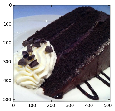
 @ interact ( n = ( 0 , len ( X_train )))
def show_pic ( n ):
    plt . imshow ( X_train [ n ])
    print ( 'class:' , y_train [ n ], ix_to_class [ y_train [ n ]])
class: 21 chocolate_cake
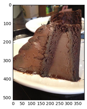
 @ interact ( n = ( 0 , len ( X_test )))
def show_pic ( n ):
    plt . imshow ( X_test [ n ])
    print ( 'class:' , y_test [ n ], ix_to_class [ y_test [ n ]])
class: 21 chocolate_cake
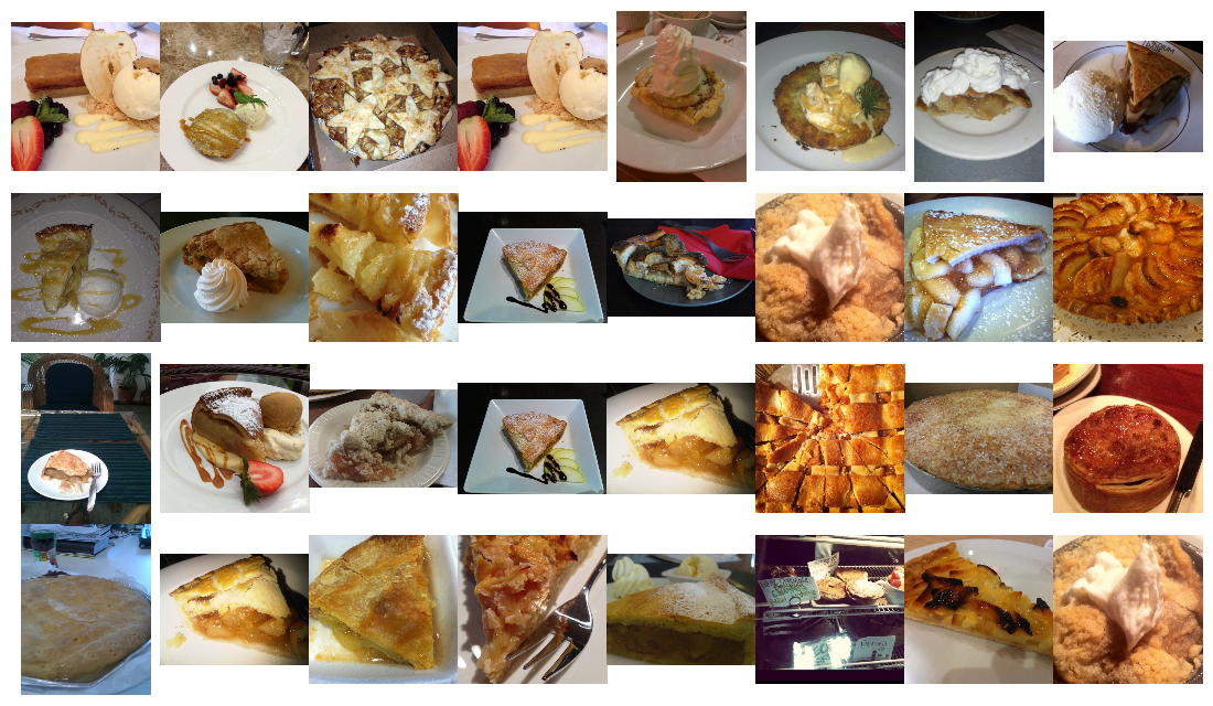
 @ interact ( n_class = sorted_class_to_ix )
def show_random_images_of_class ( n_class = 0 ):
    print ( n_class )
    nrows = 4
    ncols = 8
    fig , axes = plt . subplots ( nrows = nrows , ncols = ncols )
    fig . set_size_inches ( 12 , 8 )
    #fig.tight_layout()
    imgs = np . random . choice (( y_train == n_class ). nonzero ()[ 0 ], nrows * ncols )
    for i , ax in enumerate ( axes . flat ):
        im = ax . imshow ( X_train [ imgs [ i ]])
        ax . set_axis_off ()
        ax . title . set_visible ( False )
        ax . xaxis . set_ticks ([])
        ax . yaxis . set_ticks ([])
        for spine in ax . spines . values ():
            spine . set_visible ( False )
    plt . subplots_adjust ( left = 0 , wspace = 0 , hspace = 0 )
    plt . show ()
0
 @ interact ( n_class = sorted_class_to_ix )
def show_random_images_of_class ( n_class = 0 ):
    print ( n_class )
    nrows = 4
    ncols = 8
    fig , axes = plt . subplots ( nrows = nrows , ncols = ncols )
    fig . set_size_inches ( 12 , 8 )
    #fig.tight_layout()
    imgs = np . random . choice (( y_test == n_class ). nonzero ()[ 0 ], nrows * ncols )
    for i , ax in enumerate ( axes . flat ):
        im = ax . imshow ( X_test [ imgs [ i ]])
        ax . set_axis_off ()
        ax . title . set_visible ( False )
        ax . xaxis . set_ticks ([])
        ax . yaxis . set_ticks ([])
        for spine in ax . spines . values ():
            spine . set_visible ( False )
    plt . subplots_adjust ( left = 0 , wspace = 0 , hspace = 0 )
    plt . show ()
0
n_classes 값을 취할 수있는 하나의 기능이 아닌 이진 기능의 벡터를 생성하려면 각 레이블 값을 인코딩해야합니다.
 from keras . utils . np_utils import to_categorical

n_classes = 101
y_train_cat = to_categorical ( y_train , nb_classes = n_classes )
y_test_cat = to_categorical ( y_test , nb_classes = n_classes )
from keras . applications . inception_v3 import InceptionV3
from keras . applications . inception_v3 import preprocess_input , decode_predictions
from keras . preprocessing import image
from keras . layers import Input
import tools . image_gen_extended as T
# Useful for checking the output of the generators after code change
#from importlib import reload
#reload(T)Keras와 함께 배송하는 것보다 더 강력한 이미지 확대 파이프 라인이 필요했습니다. 운 좋게도, 나는이 수정 된 버전을 내베이스로 사용할 수있었습니다.
저자는 확장 가능한 파이프 라인을 추가하여 사용자 정의 자르기 기능과 같은 추가 수정을 지정하고 Inception Image Preprocessor를 사용할 수 있습니다. 모든 훈련 세트를 float32s 로 유지하기에 충분한 메모리가 없기 때문에 전처리를 동적으로 적용 할 수 있어야했습니다. 나는 전체 훈련 세트를 uint8s 로로드 할 수있었습니다.
또한 GPU 나 멀티 코어 CPU를 완전히 활용하지 않았습니다. 기본적으로 Python은 단일 코어 만 사용할 수 있으므로 교육을 위해 GPU에 보낼 수있는 처리 된/증강 이미지의 양을 제한합니다. 일부 성능 모니터링을 기반으로 GPU의 적은 비율 만 사용했습니다. 파이썬 multiprocessing Pool 통합함으로써 약 50% CPU 이용률과 90% GPU 사용을 얻을 수있었습니다.
최종 결과는 각 훈련의 각 시대가 45 분에서 22 분으로 갔다는 것입니다! 이 노트북에서 훈련하는 동안 GPU 그래프를 직접 실행할 수 있습니다. 데이터 확대 및 GPU 성능 향상에 대한 영감은 Jimmie Goode : 데이터 확대를위한 버퍼링 된 파이썬 생성기에서 나왔습니다.
현재 코드는 상당히 버그가 많으며 교육이 수동으로 중단 될 때마다 파이썬 커널을 다시 시작해야합니다. 코드는 상당히 해킹되었으며 피팅과 관련된 기능과 같은 특정 기능이 비활성화됩니다. 나는이 이미지지 게이터를 개선하고 미래에 커뮤니티에 공개하기를 희망합니다.
display ( Image ( './gpu.png' ))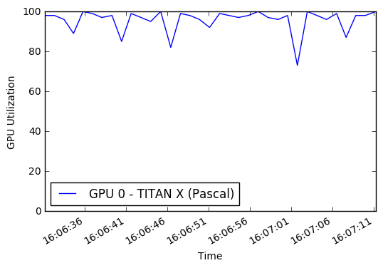
 % % time

# this is the augmentation configuration we will use for training
train_datagen = T . ImageDataGenerator (
    featurewise_center = False ,  # set input mean to 0 over the dataset
    samplewise_center = False ,  # set each sample mean to 0
    featurewise_std_normalization = False ,  # divide inputs by std of the dataset
    samplewise_std_normalization = False ,  # divide each input by its std
    zca_whitening = False ,  # apply ZCA whitening
    rotation_range = 0 ,  # randomly rotate images in the range (degrees, 0 to 180)
    width_shift_range = 0.2 ,  # randomly shift images horizontally (fraction of total width)
    height_shift_range = 0.2 ,  # randomly shift images vertically (fraction of total height)
    horizontal_flip = True ,  # randomly flip images
    vertical_flip = False , # randomly flip images
    zoom_range = [ .8 , 1 ],
    channel_shift_range = 30 ,
    fill_mode = 'reflect' )
train_datagen . config [ 'random_crop_size' ] = ( 299 , 299 )
train_datagen . set_pipeline ([ T . random_transform , T . random_crop , T . preprocess_input ])
train_generator = train_datagen . flow ( X_train , y_train_cat , batch_size = 64 , seed = 11 , pool = pool )
test_datagen = T . ImageDataGenerator ()
test_datagen . config [ 'random_crop_size' ] = ( 299 , 299 )
test_datagen . set_pipeline ([ T . random_transform , T . random_crop , T . preprocess_input ])
test_generator = test_datagen . flow ( X_test , y_test_cat , batch_size = 64 , seed = 11 , pool = pool )우리는 이러한 이미지 라테 에너터에서 어떤 종류의 이미지가 나오는지 알 수 있습니다.
 def reverse_preprocess_input ( x0 ):
    x = x0 / 2.0
    x += 0.5
    x *= 255.
    return x
% % time
@ interact ()
def show_images ( unprocess = True ):
for x in test_generator :
fig , axes = plt . subplots ( nrows = 8 , ncols = 4 )
fig . set_size_inches ( 8 , 8 )
page = 0
page_size = 32
start_i = page * page_size
for i , ax in enumerate ( axes . flat ):
img = x [ 0 ][ i + start_i ]
if unprocess :
im = ax . imshow ( reverse_preprocess_input ( img ). astype ( 'uint8' ) )
else :
im = ax . imshow ( img )
ax . set_axis_off ()
ax . title . set_visible ( False )
ax . xaxis . set_ticks ([])
ax . yaxis . set_ticks ([])
for spine in ax . spines . values ():
spine . set_visible ( False )
plt . subplots_adjust ( left = 0 , wspace = 0 , hspace = 0 )
plt . show ()
break 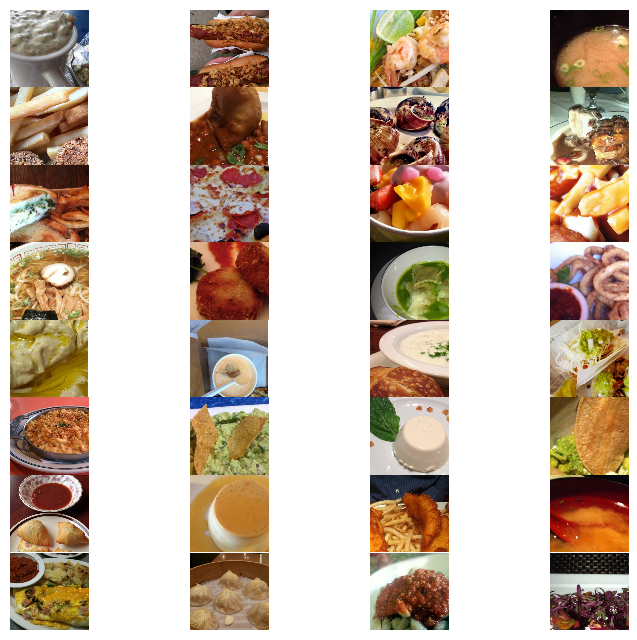
 CPU times: user 1.54 s, sys: 524 ms, total: 2.06 s
Wall time: 2.24 s
 % % time
show_images ( unprocess = False )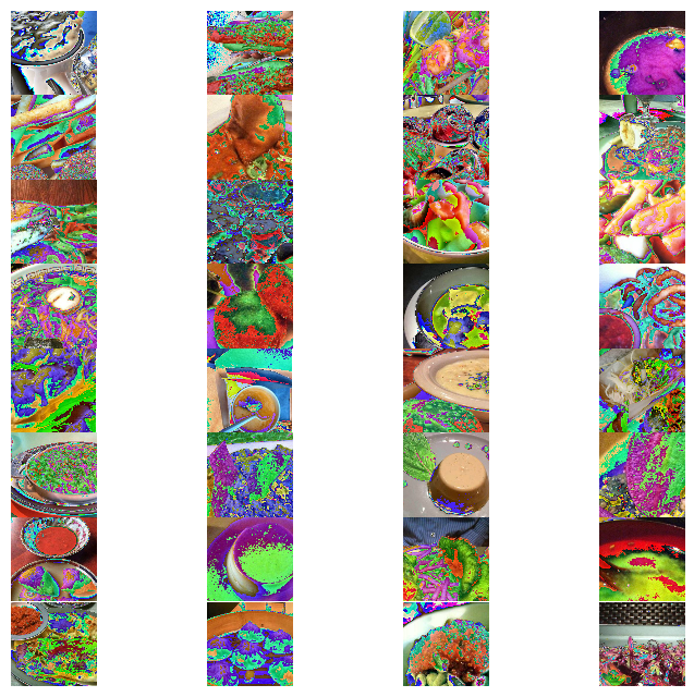
 CPU times: user 1.58 s, sys: 300 ms, total: 1.88 s
Wall time: 2.11 s
Google InceptionV3 모델을 재교육하고 ImageNet에서 사전에 재교육 할 것입니다. 신경망 아키텍처는 다음과 같습니다.
 % % time
from keras . models import Sequential , Model
from keras . layers import Dense , Dropout , Activation , Flatten
from keras . layers import Convolution2D , MaxPooling2D , ZeroPadding2D , GlobalAveragePooling2D , AveragePooling2D
from keras . layers . normalization import BatchNormalization
from keras . preprocessing . image import ImageDataGenerator
from keras . callbacks import ModelCheckpoint , CSVLogger , LearningRateScheduler , ReduceLROnPlateau
from keras . optimizers import SGD
from keras . regularizers import l2
import keras . backend as K
import math

K . clear_session ()

base_model = InceptionV3 ( weights = 'imagenet' , include_top = False , input_tensor = Input ( shape = ( 299 , 299 , 3 )))
x = base_model . output
x = AveragePooling2D ( pool_size = ( 8 , 8 ))( x )
x = Dropout ( .4 )( x )
x = Flatten ()( x )
predictions = Dense ( n_classes , init = 'glorot_uniform' , W_regularizer = l2 ( .0005 ), activation = 'softmax' )( x )

model = Model ( input = base_model . input , output = predictions )

opt = SGD ( lr = .01 , momentum = .9 )
model . compile ( optimizer = opt , loss = 'categorical_crossentropy' , metrics = [ 'accuracy' ])

checkpointer = ModelCheckpoint ( filepath = 'model4.{epoch:02d}-{val_loss:.2f}.hdf5' , verbose = 1 , save_best_only = True )
csv_logger = CSVLogger ( 'model4.log' )

def schedule ( epoch ):
    if epoch < 15 :
        return .01
    elif epoch < 28 :
        return .002
    else :
        return .0004
lr_scheduler = LearningRateScheduler ( schedule )

model . fit_generator ( train_generator ,
                    validation_data = test_generator ,
                    nb_val_samples = X_test . shape [ 0 ],
                    samples_per_epoch = X_train . shape [ 0 ],
                    nb_epoch = 32 ,
                    verbose = 2 ,
                    callbacks = [ lr_scheduler , csv_logger , checkpointer ])
Epoch 1/32
Epoch 00000: val_loss improved from inf to 3.37355, saving model to model4.00-3.37.hdf5
1342s - loss: 4.2541 - acc: 0.0810 - val_loss: 3.3736 - val_acc: 0.2010
Epoch 2/32
Epoch 00001: val_loss improved from 3.37355 to 2.36625, saving model to model4.01-2.37.hdf5
1329s - loss: 2.9745 - acc: 0.3075 - val_loss: 2.3662 - val_acc: 0.4071
Epoch 3/32
Epoch 00002: val_loss improved from 2.36625 to 1.79355, saving model to model4.02-1.79.hdf5
1329s - loss: 2.3080 - acc: 0.4539 - val_loss: 1.7935 - val_acc: 0.5338
Epoch 4/32
Epoch 00003: val_loss improved from 1.79355 to 1.48898, saving model to model4.03-1.49.hdf5
1356s - loss: 2.0102 - acc: 0.5216 - val_loss: 1.4890 - val_acc: 0.6068
Epoch 5/32
Epoch 00004: val_loss improved from 1.48898 to 1.34121, saving model to model4.04-1.34.hdf5
1330s - loss: 1.8436 - acc: 0.5577 - val_loss: 1.3412 - val_acc: 0.6431
Epoch 6/32
Epoch 00005: val_loss improved from 1.34121 to 1.22485, saving model to model4.05-1.22.hdf5
1329s - loss: 1.7057 - acc: 0.5909 - val_loss: 1.2248 - val_acc: 0.6740
Epoch 7/32
Epoch 00006: val_loss did not improve
1328s - loss: 1.5996 - acc: 0.6126 - val_loss: 1.2310 - val_acc: 0.6716
Epoch 8/32
Epoch 00007: val_loss improved from 1.22485 to 1.11248, saving model to model4.07-1.11.hdf5
1331s - loss: 1.5148 - acc: 0.6314 - val_loss: 1.1125 - val_acc: 0.7022
Epoch 9/32
Epoch 00008: val_loss improved from 1.11248 to 1.07145, saving model to model4.08-1.07.hdf5
1331s - loss: 1.4395 - acc: 0.6506 - val_loss: 1.0714 - val_acc: 0.7095
Epoch 10/32
Epoch 00009: val_loss improved from 1.07145 to 1.05129, saving model to model4.09-1.05.hdf5
1333s - loss: 1.3900 - acc: 0.6637 - val_loss: 1.0513 - val_acc: 0.7181
Epoch 11/32
Epoch 00010: val_loss improved from 1.05129 to 1.03356, saving model to model4.10-1.03.hdf5
1331s - loss: 1.3316 - acc: 0.6780 - val_loss: 1.0336 - val_acc: 0.7250
Epoch 12/32
Epoch 00011: val_loss improved from 1.03356 to 1.00622, saving model to model4.11-1.01.hdf5
1331s - loss: 1.2850 - acc: 0.6893 - val_loss: 1.0062 - val_acc: 0.7275
Epoch 13/32
Epoch 00012: val_loss improved from 1.00622 to 0.94016, saving model to model4.12-0.94.hdf5
1330s - loss: 1.2325 - acc: 0.7003 - val_loss: 0.9402 - val_acc: 0.7461
Epoch 14/32
Epoch 00013: val_loss did not improve
1330s - loss: 1.1970 - acc: 0.7086 - val_loss: 0.9461 - val_acc: 0.7453
Epoch 15/32
Epoch 00014: val_loss did not improve
1329s - loss: 1.1683 - acc: 0.7154 - val_loss: 0.9691 - val_acc: 0.7396
Epoch 16/32
Epoch 00015: val_loss improved from 0.94016 to 0.71776, saving model to model4.15-0.72.hdf5
1329s - loss: 0.9398 - acc: 0.7724 - val_loss: 0.7178 - val_acc: 0.8055
Epoch 17/32
Epoch 00016: val_loss improved from 0.71776 to 0.70245, saving model to model4.16-0.70.hdf5
1329s - loss: 0.8591 - acc: 0.7916 - val_loss: 0.7025 - val_acc: 0.8069
Epoch 18/32
Epoch 00017: val_loss did not improve
1327s - loss: 0.8238 - acc: 0.8023 - val_loss: 0.7093 - val_acc: 0.8053
Epoch 19/32
Epoch 00018: val_loss did not improve
1327s - loss: 0.7947 - acc: 0.8093 - val_loss: 0.7048 - val_acc: 0.8059
Epoch 20/32
Epoch 00019: val_loss did not improve
1327s - loss: 0.7713 - acc: 0.8143 - val_loss: 0.7097 - val_acc: 0.8061
Epoch 21/32
Epoch 00020: val_loss improved from 0.70245 to 0.69545, saving model to model4.20-0.70.hdf5
1329s - loss: 0.7458 - acc: 0.8195 - val_loss: 0.6955 - val_acc: 0.8104
Epoch 22/32
Epoch 00021: val_loss did not improve
1328s - loss: 0.7282 - acc: 0.8232 - val_loss: 0.6977 - val_acc: 0.8119
Epoch 23/32
Epoch 00022: val_loss improved from 0.69545 to 0.69190, saving model to model4.22-0.69.hdf5
1328s - loss: 0.7114 - acc: 0.8284 - val_loss: 0.6919 - val_acc: 0.8150
Epoch 24/32
Epoch 00023: val_loss did not improve
1325s - loss: 0.6983 - acc: 0.8311 - val_loss: 0.7002 - val_acc: 0.8116
Epoch 25/32
Epoch 00024: val_loss did not improve
1330s - loss: 0.6719 - acc: 0.8381 - val_loss: 0.7031 - val_acc: 0.8112
Epoch 26/32
Epoch 00025: val_loss did not improve
1382s - loss: 0.6607 - acc: 0.8407 - val_loss: 0.7115 - val_acc: 0.8083
Epoch 27/32
Epoch 00026: val_loss did not improve
1330s - loss: 0.6479 - acc: 0.8439 - val_loss: 0.7037 - val_acc: 0.8126
Epoch 28/32
Epoch 00027: val_loss did not improve
1328s - loss: 0.6292 - acc: 0.8478 - val_loss: 0.7122 - val_acc: 0.8086
Epoch 29/32
Epoch 00028: val_loss improved from 0.69190 to 0.68908, saving model to model4.28-0.69.hdf5
1330s - loss: 0.5983 - acc: 0.8580 - val_loss: 0.6891 - val_acc: 0.8165
Epoch 30/32
Epoch 00029: val_loss improved from 0.68908 to 0.68740, saving model to model4.29-0.69.hdf5
1330s - loss: 0.5817 - acc: 0.8612 - val_loss: 0.6874 - val_acc: 0.8149
Epoch 31/32
Epoch 00030: val_loss did not improve
1328s - loss: 0.5729 - acc: 0.8642 - val_loss: 0.6912 - val_acc: 0.8143
Epoch 32/32
Epoch 00031: val_loss did not improve
1329s - loss: 0.5638 - acc: 0.8663 - val_loss: 0.6895 - val_acc: 0.8159
CPU times: user 8h 49min 20s, sys: 1h 55min 54s, total: 10h 45min 14s
Wall time: 11h 51min 18s
이 시점에서, 우리는 테스트 세트에서 최대 81.65 개의 단일 작물 상단 정확도를보고 있습니다. 우리는 더 느린 학습 속도로 모델을 계속 교육하여 더 많은 개선을 할 수 있습니다.
저의 초기 실험은 Adam 및 Adadelta와 같은보다 현대적인 최적화기와 더 높은 학습 률을 사용했습니다. 나는 문헌을 더 밀접하게 따르기로 결정하고 학습 일정이 빠르게 감소 된 확률 론적 그라디언트 하강 (SGD)을 사용하기 전에 80% 이하의 정확도를 한동안 멈췄다. 우리가 다차원 표면을 검색 할 때 때로는 느리게 진행되는 것이 먼 길을갑니다.
멀티 프로세싱 코드의 불안정성으로 인해 때로는 노트북을 다시 시작하고 최신 모델을로드 한 다음 계속 교육해야합니다.
 % % time
from keras . models import Sequential , Model , load_model
from keras . layers import Dense , Dropout , Activation , Flatten
from keras . layers import Convolution2D , MaxPooling2D , ZeroPadding2D , GlobalAveragePooling2D , AveragePooling2D
from keras . layers . normalization import BatchNormalization
from keras . preprocessing . image import ImageDataGenerator
from keras . callbacks import ModelCheckpoint , CSVLogger , LearningRateScheduler , ReduceLROnPlateau
from keras . optimizers import SGD
from keras . regularizers import l2
import keras . backend as K
import math

model = load_model ( filepath = './model4.29-0.69.hdf5' )

opt = SGD ( lr = .01 , momentum = .9 )
model . compile ( optimizer = opt , loss = 'categorical_crossentropy' , metrics = [ 'accuracy' ])

checkpointer = ModelCheckpoint ( filepath = 'model4b.{epoch:02d}-{val_loss:.2f}.hdf5' , verbose = 1 , save_best_only = True )
csv_logger = CSVLogger ( 'model4b.log' )

def schedule ( epoch ):
    if epoch < 10 :
        return .00008
    elif epoch < 20 :
        return .000016
    else :
        return .0000032

lr_scheduler = LearningRateScheduler ( schedule )

model . fit_generator ( train_generator ,
                    validation_data = test_generator ,
                    nb_val_samples = X_test . shape [ 0 ],
                    samples_per_epoch = X_train . shape [ 0 ],
                    nb_epoch = 32 ,
                    verbose = 2 ,
callbacks = [ lr_scheduler , csv_logger , checkpointer ]) 이 시점에서 디스크에 여러 훈련 된 모델을 저장해야합니다. 우리는 그것들을 통과하고 load_model 함수를 사용하여 가장 낮은 손실 / 가장 높은 정확도로 모델을로드 할 수 있습니다.
 % % time
#model = load_model(filepath='./model4.29-0.69.hdf5') # 86.8039 10-crop Top-1 test accuracy
model = load_model ( filepath = './model4b.10-0.68.hdf5' ) # 86.9703
CPU times: user 36.4 s, sys: 1.11 s, total: 37.5 s
Wall time: 36.5 s
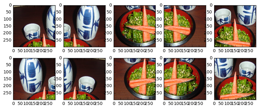
또한 여러 작물을 사용하여 테스트 세트를 평가하려고합니다. 이는 단일 작물 평가에 비해 5%의 정확도 향상을 일으킬 수 있습니다. 다음 작물을 사용하는 것이 일반적입니다 : 왼쪽 상단, 오른쪽 상단, 왼쪽 아래, 오른쪽 아래, 중앙. 우리는 또한 이미지에서 같은 작물을 왼쪽에서 오른쪽으로 뒤집어 총 10 개의 작물을 만듭니다.
또한, 예를 들어 상위 5 개의 정확도를 계산하기 위해 각 작물에 대한 최상위 예측을 반환하려고합니다.
 def center_crop ( x , center_crop_size , ** kwargs ):
    centerw , centerh = x . shape [ 0 ] // 2 , x . shape [ 1 ] // 2
    halfw , halfh = center_crop_size [ 0 ] // 2 , center_crop_size [ 1 ] // 2
    return x [ centerw - halfw : centerw + halfw + 1 , centerh - halfh : centerh + halfh + 1 , :]
def predict_10_crop ( img , ix , top_n = 5 , plot = False , preprocess = True , debug = False ):
flipped_X = np . fliplr ( img )
crops = [
img [: 299 ,: 299 , :], # Upper Left
img [: 299 , img . shape [ 1 ] - 299 :, :], # Upper Right
img [ img . shape [ 0 ] - 299 :, : 299 , :], # Lower Left
img [ img . shape [ 0 ] - 299 :, img . shape [ 1 ] - 299 :, :], # Lower Right
center_crop ( img , ( 299 , 299 )),
flipped_X [: 299 ,: 299 , :],
flipped_X [: 299 , flipped_X . shape [ 1 ] - 299 :, :],
flipped_X [ flipped_X . shape [ 0 ] - 299 :, : 299 , :],
flipped_X [ flipped_X . shape [ 0 ] - 299 :, flipped_X . shape [ 1 ] - 299 :, :],
center_crop ( flipped_X , ( 299 , 299 ))
]
if preprocess :
crops = [ preprocess_input ( x . astype ( 'float32' )) for x in crops ]
if plot :
fig , ax = plt . subplots ( 2 , 5 , figsize = ( 10 , 4 ))
ax [ 0 ][ 0 ]. imshow ( crops [ 0 ])
ax [ 0 ][ 1 ]. imshow ( crops [ 1 ])
ax [ 0 ][ 2 ]. imshow ( crops [ 2 ])
ax [ 0 ][ 3 ]. imshow ( crops [ 3 ])
ax [ 0 ][ 4 ]. imshow ( crops [ 4 ])
ax [ 1 ][ 0 ]. imshow ( crops [ 5 ])
ax [ 1 ][ 1 ]. imshow ( crops [ 6 ])
ax [ 1 ][ 2 ]. imshow ( crops [ 7 ])
ax [ 1 ][ 3 ]. imshow ( crops [ 8 ])
ax [ 1 ][ 4 ]. imshow ( crops [ 9 ])
y_pred = model . predict ( np . array ( crops ))
preds = np . argmax ( y_pred , axis = 1 )
top_n_preds = np . argpartition ( y_pred , - top_n )[:, - top_n :]
if debug :
print ( 'Top-1 Predicted:' , preds )
print ( 'Top-5 Predicted:' , top_n_preds )
print ( 'True Label:' , y_test [ ix ])
return preds , top_n_preds
ix = 13001
predict_10_crop ( X_test [ ix ], ix , top_n = 5 , plot = True , preprocess = False , debug = True ) Top-1 Predicted: [74 74 74 74 74 74 74 74 74 74]
Top-5 Predicted: [[33 97 37 39 74]
[28 52 37 39 74]
[73 39 52 37 74]
[35 33 37 39 74]
[35 33 37 39 74]
[35 33 37 39 74]
[35 33 37 39 74]
[97 37 73 39 74]
[73 52 37 39 74]
[34 35 33 39 74]]
True Label: 88
(array([74, 74, 74, 74, 74, 74, 74, 74, 74, 74]), array([[33, 97, 37, 39, 74],
[28, 52, 37, 39, 74],
[73, 39, 52, 37, 74],
[35, 33, 37, 39, 74],
[35, 33, 37, 39, 74],
[35, 33, 37, 39, 74],
[35, 33, 37, 39, 74],
[97, 37, 73, 39, 74],
[73, 52, 37, 39, 74],
[34, 35, 33, 39, 74]]))
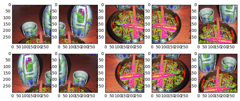
또한 Inception 모델의 이미지를 전처리해야합니다.
 ix = 13001
predict_10_crop ( X_test [ ix ], ix , top_n = 5 , plot = True , preprocess = True , debug = True )
Top-1 Predicted: [51 51 88 88 88 51 51 88 88 88]
Top-5 Predicted: [[18 79 51 13 48]
[48 79 11 55 51]
[79 93 81 37 88]
[51 86 93 81 88]
[11 79 51 81 88]
[19 79 51 56 13]
[11 88 48 51 13]
[37 93 86 88 81]
[37 79 93 88 81]
[84 81 11 79 88]]
True Label: 88
(array([51, 51, 88, 88, 88, 51, 51, 88, 88, 88]), array([[18, 79, 51, 13, 48],
[48, 79, 11, 55, 51],
[79, 93, 81, 37, 88],
[51, 86, 93, 81, 88],
[11, 79, 51, 81, 88],
[19, 79, 51, 56, 13],
[11, 88, 48, 51, 13],
[37, 93, 86, 88, 81],
[37, 79, 93, 88, 81],
[84, 81, 11, 79, 88]]))
이제 테스트 세트에서 각 항목에 대한 작물을 만들고 예측을받습니다. 다중 프로세싱 또는 다른 유형의 병렬 처리를 이용하지 않기 때문에 이것은 현재 느린 과정입니다.
 % % time
preds_10_crop = {}
for ix in range ( len ( X_test )):
    if ix % 1000 == 0 :
        print ( ix )
    preds_10_crop [ ix ] = predict_10_crop ( X_test [ ix ], ix )
0
1000
2000
3000
4000
5000
6000
7000
8000
9000
10000
11000
12000
13000
14000
15000
16000
17000
18000
19000
20000
21000
22000
23000
24000
25000
CPU times: user 50min 3s, sys: 5min 13s, total: 55min 16s
Wall time: 31min 28s
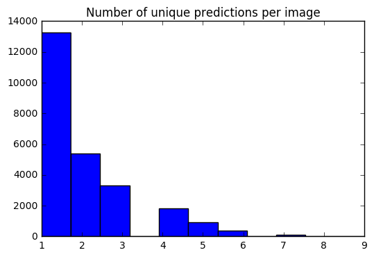
이제 각 이미지에 대해 10 가지 예측 세트가 있습니다. 히스토그램을 사용하여 각 이미지에 대한 고유 한 예측의 #이 어떻게 배포되는지 확인할 수 있습니다.
 preds_uniq = { k : np . unique ( v [ 0 ]) for k , v in preds_10_crop . items ()}
preds_hist = np . array ([ len ( x ) for x in preds_uniq . values ()])

plt . hist ( preds_hist , bins = 11 )
plt . title ( 'Number of unique predictions per image' )
<matplotlib.text.Text at 0x7fe30c3daa20>
테스트 항목 인덱스를 Top-1 / Top-5 예측에 매핑하기위한 사전을 만들어 봅시다.
 preds_top_1 = { k : collections . Counter ( v [ 0 ]). most_common ( 1 ) for k , v in preds_10_crop . items ()}

top_5_per_ix = { k : collections . Counter ( preds_10_crop [ k ][ 1 ]. reshape ( - 1 )). most_common ( 5 )
                for k , v in preds_10_crop . items ()}
preds_top_5 = { k : [ y [ 0 ] for y in v ] for k , v in top_5_per_ix . items ()}
% % time
right_counter = 0
for i in range ( len ( y_test )):
guess , actual = preds_top_1 [ i ][ 0 ][ 0 ], y_test [ i ]
if guess == actual :
right_counter += 1
print ( 'Top-1 Accuracy, 10-Crop: {0:.2f}%' . format ( right_counter / len ( y_test ) * 100 )) Top-1 Accuracy, 10-Crop: 86.97%
CPU times: user 28 ms, sys: 0 ns, total: 28 ms
Wall time: 27.3 ms
 % % time
top_5_counter = 0
for i in range ( len ( y_test )):
    guesses , actual = preds_top_5 [ i ], y_test [ i ]
    if actual in guesses :
        top_5_counter += 1

print ( 'Top-5 Accuracy, 10-Crop: {0:.2f}%' . format ( top_5_counter / len ( y_test ) * 100 ))
Top-5 Accuracy, 10-Crop: 97.42%
CPU times: user 28 ms, sys: 0 ns, total: 28 ms
Wall time: 27 ms
y_pred = [ x [ 0 ][ 0 ] for x in preds_top_1 . values ()] @ interact ( page = [ 0 , int ( len ( X_test ) / 20 )])
def show_images_prediction ( page = 0 ):
page_size = 20
nrows = 4
ncols = 5
fig , axes = plt . subplots ( nrows = nrows , ncols = ncols , figsize = ( 12 , 12 ))
fig . set_size_inches ( 12 , 8 )
#fig.tight_layout()
#imgs = np.random.choice((y_all == n_class).nonzero()[0], nrows * ncols)
start_i = page * page_size
for i , ax in enumerate ( axes . flat ):
im = ax . imshow ( X_test [ i + start_i ])
ax . set_axis_off ()
ax . title . set_visible ( False )
ax . xaxis . set_ticks ([])
ax . yaxis . set_ticks ([])
for spine in ax . spines . values ():
spine . set_visible ( False )
predicted = ix_to_class [ y_pred [ i + start_i ]]
match = predicted == ix_to_class [ y_test [ start_i + i ]]
ec = ( 1 , .5 , .5 )
fc = ( 1 , .8 , .8 )
if match :
ec = ( 0 , .6 , .1 )
fc = ( 0 , .7 , .2 )
# predicted label
ax . text ( 0 , 400 , 'P: ' + predicted , size = 10 , rotation = 0 ,
ha = "left" , va = "top" ,
bbox = dict ( boxstyle = "round" ,
ec = ec ,
fc = fc ,
)
)
if not match :
# true label
ax . text ( 0 , 480 , 'A: ' + ix_to_class [ y_test [ start_i + i ]], size = 10 , rotation = 0 ,
ha = "left" , va = "top" ,
bbox = dict ( boxstyle = "round" ,
ec = ec ,
fc = fc ,
)
)
plt . subplots_adjust ( left = 0 , wspace = 1 , hspace = 0 )
plt . show ()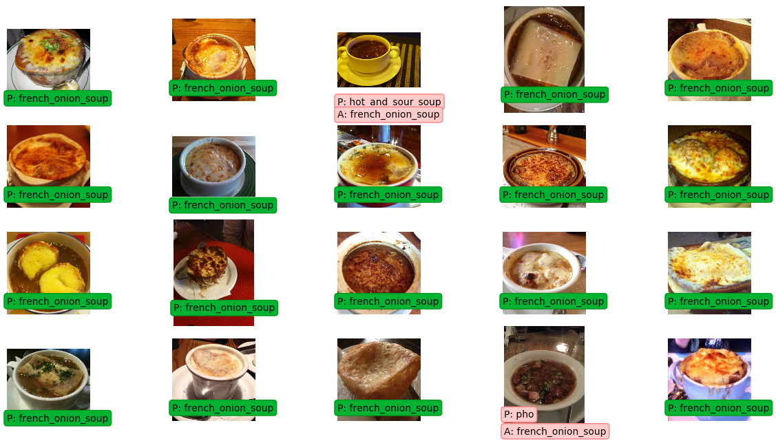
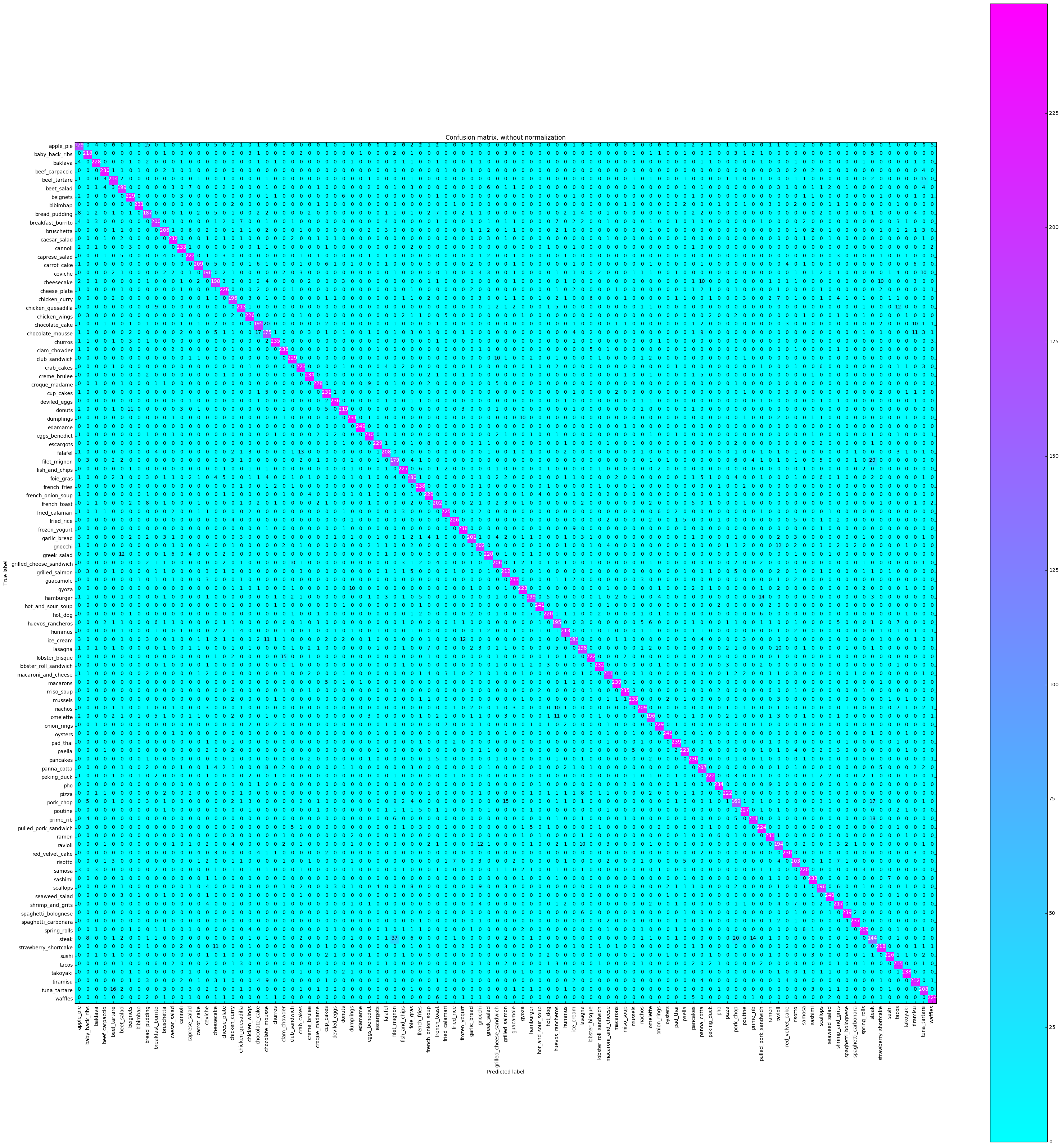
혼란 매트릭스는 각 클래스 레이블을 플로팅하며 다른 시간은 다른 클래스로 올바르게 레이블을 붙였습니다.
 % % time
from sklearn . metrics import confusion_matrix
import itertools

def plot_confusion_matrix ( cm , classes ,
                          normalize = False ,
                          title = 'Confusion matrix' ,
                          cmap = plt . cm . Blues ):
    """
    This function prints and plots the confusion matrix.
    Normalization can be applied by setting `normalize=True`.
    """
    plt . imshow ( cm , interpolation = 'nearest' , cmap = cmap )
    plt . title ( title )
    plt . colorbar ()
    tick_marks = np . arange ( len ( classes ))
    plt . xticks ( tick_marks , classes , rotation = 90 )
    plt . yticks ( tick_marks , classes )

    if normalize :
        cm = cm . astype ( 'float' ) / cm . sum ( axis = 1 )[:, np . newaxis ]
        print ( "Normalized confusion matrix" )
    else :
        print ( 'Confusion matrix, without normalization' )

    print ( cm )

    thresh = cm . max () / 2.
    for i , j in itertools . product ( range ( cm . shape [ 0 ]), range ( cm . shape [ 1 ])):
        plt . text ( j , i , cm [ i , j ],
                 horizontalalignment = "center" ,
                 color = "white" if cm [ i , j ] > thresh else "black" )

    plt . tight_layout ()
    plt . ylabel ( 'True label' )
    plt . xlabel ( 'Predicted label' )


# Compute confusion matrix
cnf_matrix = confusion_matrix ( y_test , y_pred )
np . set_printoptions ( precision = 2 )

class_names = [ ix_to_class [ i ] for i in range ( 101 )]

plt . figure ()
fig = plt . gcf ()
fig . set_size_inches ( 32 , 32 )
plot_confusion_matrix ( cnf_matrix , classes = class_names ,
                      title = 'Confusion matrix, without normalization' ,
                      cmap = plt . cm . cool )
plt . show ()
Confusion matrix, without normalization
[[179 0 4 ..., 2 0 5]
[ 0 218 0 ..., 0 0 0]
[ 4 0 228 ..., 1 0 0]
...,
[ 0 0 0 ..., 212 0 1]
[ 0 0 0 ..., 0 208 0]
[ 0 0 0 ..., 0 0 224]]
 CPU times: user 16.4 s, sys: 1.22 s, total: 17.6 s
Wall time: 16.4 s
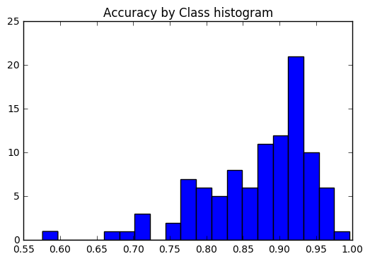
우리는 정확도가 모든 클래스에서 일관성이 있는지 또는 일부 클래스가 다른 클래스보다 훨씬 쉽게 레이블을 지정하는지 확인하고 싶습니다. 우리의 음모에 따르면, 몇 가지 클래스는 올바르게 레이블을 지정하기가 훨씬 더 어려워지는 특이 치였습니다.
 corrects = collections . defaultdict ( int )
incorrects = collections . defaultdict ( int )
for ( pred , actual ) in zip ( y_pred , y_test ):
    if pred == actual :
        corrects [ actual ] += 1
    else :
        incorrects [ actual ] += 1

class_accuracies = {}
for ix in range ( 101 ):
    class_accuracies [ ix ] = corrects [ ix ] / 250

plt . hist ( list ( class_accuracies . values ()), bins = 20 )
plt . title ( 'Accuracy by Class histogram' )
<matplotlib.text.Text at 0x7fe2d5d4f860>
 sorted_class_accuracies = sorted ( class_accuracies . items (), key = lambda x : - x [ 1 ])
[( ix_to_class [ c [ 0 ]], c [ 1 ]) for c in sorted_class_accuracies ]
[('edamame', 0.996),
('hot_and_sour_soup', 0.964),
('oysters', 0.964),
('seaweed_salad', 0.96),
('macarons', 0.956),
('pad_thai', 0.956),
('spaghetti_bolognese', 0.956),
('french_fries', 0.952),
('frozen_yogurt', 0.952),
('takoyaki', 0.952),
('spaghetti_carbonara', 0.948),
('clam_chowder', 0.944),
('deviled_eggs', 0.944),
('churros', 0.94),
('miso_soup', 0.94),
('creme_brulee', 0.936),
('pho', 0.936),
('cannoli', 0.932),
('guacamole', 0.932),
('mussels', 0.932),
('sashimi', 0.932),
('caesar_salad', 0.928),
('lobster_roll_sandwich', 0.928),
('bibimbap', 0.924),
('cup_cakes', 0.924),
('dumplings', 0.924),
('ramen', 0.924),
('beef_carpaccio', 0.92),
('eggs_benedict', 0.92),
('pancakes', 0.92),
('red_velvet_cake', 0.92),
('beignets', 0.916),
('club_sandwich', 0.916),
('escargots', 0.916),
('french_onion_soup', 0.916),
('onion_rings', 0.916),
('baklava', 0.912),
('croque_madame', 0.912),
('fish_and_chips', 0.908),
('poutine', 0.908),
('cheese_plate', 0.904),
('chicken_wings', 0.904),
('fried_rice', 0.904),
('sushi', 0.904),
('fried_calamari', 0.9),
('pulled_pork_sandwich', 0.896),
('waffles', 0.896),
('crab_cakes', 0.892),
('gyoza', 0.892),
('paella', 0.892),
('caprese_salad', 0.888),
('lobster_bisque', 0.888),
('peking_duck', 0.888),
('pizza', 0.888),
('greek_salad', 0.88),
('hot_dog', 0.88),
('samosa', 0.88),
('donuts', 0.876),
('spring_rolls', 0.876),
('baby_back_ribs', 0.872),
('strawberry_shortcake', 0.872),
('shrimp_and_grits', 0.868),
('tacos', 0.86),
('beef_tartare', 0.856),
('prime_rib', 0.856),
('chicken_quesadilla', 0.852),
('hummus', 0.852),
('grilled_salmon', 0.848),
('tiramisu', 0.848),
('macaroni_and_cheese', 0.844),
('carrot_cake', 0.836),
('nachos', 0.836),
('falafel', 0.832),
('tuna_tartare', 0.832),
('panna_cotta', 0.828),
('bruschetta', 0.824),
('grilled_cheese_sandwich', 0.824),
('risotto', 0.812),
('french_toast', 0.808),
('gnocchi', 0.808),
('garlic_bread', 0.804),
('breakfast_burrito', 0.8),
('beet_salad', 0.796),
('hamburger', 0.796),
('cheesecake', 0.792),
('lasagna', 0.792),
('ceviche', 0.784),
('chicken_curry', 0.784),
('omelette', 0.784),
('scallops', 0.784),
('chocolate_cake', 0.78),
('huevos_rancheros', 0.78),
('ravioli', 0.776),
('ice_cream', 0.764),
('bread_pudding', 0.748),
('foie_gras', 0.72),
('apple_pie', 0.716),
('filet_mignon', 0.716),
('chocolate_mousse', 0.7),
('pork_chop', 0.676),
('steak', 0.576)]
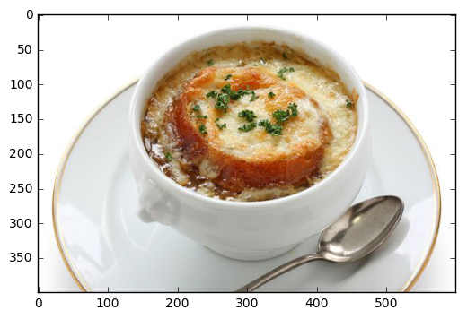
로컬 파일에서 예측
 pic_path = '/home/stratospark/Downloads/soup.jpg'
pic = img . imread ( pic_path )
preds = predict_10_crop ( np . array ( pic ), 0 )[ 0 ]
best_pred = collections . Counter ( preds ). most_common ( 1 )[ 0 ][ 0 ]
print ( ix_to_class [ best_pred ])
plt . imshow ( pic )
french_onion_soup
<matplotlib.image.AxesImage at 0x7fe2d59eb5c0>
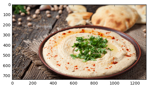
인터넷의 이미지에서 예측
 import urllib . request

@ interact
def predict_remote_image ( url = 'http://themodelhouse.tv/wp-content/uploads/2016/08/hummus.jpg' ):
    with urllib . request . urlopen ( url ) as f :
        pic = plt . imread ( f , format = 'jpg' )
        preds = predict_10_crop ( np . array ( pic ), 0 )[ 0 ]
        best_pred = collections . Counter ( preds ). most_common ( 1 )[ 0 ][ 0 ]
        print ( ix_to_class [ best_pred ])
        plt . imshow ( pic )
hummus
 with open ( 'model.json' , 'w' ) as f :
    f . write ( model . to_json ())
import json
json . dumps ( ix_to_class ) '{"0": "apple_pie", "1": "baby_back_ribs", "2": "baklava", "3": "beef_carpaccio", "4": "beef_tartare", "5": "beet_salad", "6": "beignets", "7": "bibimbap", "8": "bread_pudding", "9": "breakfast_burrito", "10": "bruschetta", "11": "caesar_salad", "12": "cannoli", "13": "caprese_salad", "14": "carrot_cake", "15": "ceviche", "16": "cheesecake", "17": "cheese_plate", "18": "chicken_curry", "19": "chicken_quesadilla", "20": "chicken_wings", "21": "chocolate_cake", "22": "chocolate_mousse", "23": "churros", "24": "clam_chowder", "25": "club_sandwich", "26": "crab_cakes", "27": "creme_brulee", "28": "croque_madame", "29": "cup_cakes", "30": "deviled_eggs", "31": "donuts", "32": "dumplings", "33": "edamame", "34": "eggs_benedict", "35": "escargots", "36": "falafel", "37": "filet_mignon", "38": "fish_and_chips", "39": "foie_gras", "40": "french_fries", "41": "french_onion_soup", "42": "french_toast", "43": "fried_calamari", "44": "fried_rice", "45": "frozen_yogurt", "46": "garlic_bread", "47": "gnocchi", "48": "greek_salad", "49": "grilled_cheese_sandwich", "50": "grilled_salmon", "51": "guacamole", "52": "gyoza", "53": "hamburger", "54": "hot_and_sour_soup", "55": "hot_dog", "56": "huevos_rancheros", "57": "hummus", "58": "ice_cream", "59": "lasagna", "60": "lobster_bisque", "61": "lobster_roll_sandwich", "62": "macaroni_and_cheese", "63": "macarons", "64": "miso_soup", "65": "mussels", "66": "nachos", "67": "omelette", "68": "onion_rings", "69": "oysters", "70": "pad_thai", "71": "paella", "72": "pancakes", "73": "panna_cotta", "74": "peking_duck", "75": "pho", "76": "pizza", "77": "pork_chop", "78": "poutine", "79": "prime_rib", "80": "pulled_pork_sandwich", "81": "ramen", "82": "ravioli", "83": "red_velvet_cake", "84": "risotto", "85": "samosa", "86": "sashimi", "87": "scallops", "88": "seaweed_salad", "89": "shrimp_and_grits", "90": "spaghetti_bolognese", "91": "spaghetti_carbonara", "92": "spring_rolls", "93": "steak", "94": "strawberry_shortcake", "95": "sushi", "96": "tacos", "97": "takoyaki", "98": "tiramisu", "99": "tuna_tartare", "100": "waffles"}'


