food 101 keras
1.0.0
 from IPython . display import HTML , Image

url = 'http://stratospark.com/demos/food-101/'
el = '<' + 'iframe src="{}"' . format ( url ) + ' width="100%" height=600></iframe>' # prevent notebook render bug
HTML ( el )Githubでこれを読んでいる場合、デモは次のようになります。以下のリンクをフォローして、私のブログでライブデモをご覧ください。
Image ( 'demo.jpg' )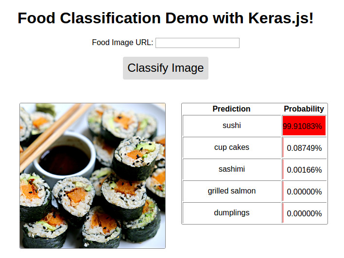
DEMO利用可能 @ http://blog.stratospark.com/deep-learning-applied-food-classification-deep-learning-keras.html
コード利用可能 @ https://github.com/stratospark/food-101-keras
更新
より広い深い学習分野内の手法である畳み込みニューラルネットワーク(CNN)は、特に過去の半年ほどでは、コンピュータービジョンアプリケーションの革新的な力でした。主なユースケースの1つは、画像分類の使用ケースです。たとえば、絵が犬か猫のものかを判断する例です。
もちろん、自分自身をバイナリ分類子に限定する必要はありません。 CNNは、コンピュータービジョンアルゴリズムのパフォーマンスのベンチマークに使用される、1000クラスのよく知られているImagenetデータセットに見られるように、数千の異なるクラスに簡単にスケーリングできます。
過去数年で、これらの最先端のテクニックは、より広範なソフトウェア開発コミュニティが利用できるようになり始めています。 Tensorflowなどの産業強度パッケージは、Googleがクラウド内のスケーラブルなクラスターに埋め込み/モバイルデバイスのディープラーニングアプリケーションを作成するために使用するのと同じビルディングブロックを提供しています - GPUマトリックス操作、部分微分勾配、および確率的オプティマイゼーターを手コードする必要はありませんこれにより、効率的なアプリケーションが可能になります。
このすべてに加えて、KerasなどのユーザーフレンドリーなAPIがあり、低レベルの詳細の一部を抽象化し、深い学習計算グラフの迅速なプロトタイピングに集中できるようになります。 LEGOSを混ぜて一致させて、望ましい結果を得るのと同じように。
自分の紹介プロジェクトとして、私はケラスに付属する事前に訓練された画像分類子を使用し、それを興味深いと思うデータセットで再訓練することにしました。私はおいしい料理と家庭料理にとても興味があるので、それらの線に沿った何かが食欲をそそりました。
この論文では、Food-101 - ランダムな森林を持つ採掘識別成分を採掘すると、Food-101データセットが導入されています。 101種類のクラスには食品があり、クラスごとに1000のラベル付き画像が監視されたトレーニングに利用できます。
私はこのKerasのブログ投稿に触発されました。データのほとんどを使用して強力な画像分類モデルを構築し、Github:Keras-finetuningで見つけた関連するスクリプトを構築しました。
私は最近、深い学習を実験する目的でシステムを構築しました。重要なコンポーネントは、メモリの12 GB、システムRAMの96 GB、および12コアIntel Core I7のNvidia Titan X Pascal Pascalです。 64ビットUbuntu 16.04を実行し、Anaconda Python Distributionを使用しています。残念ながら、十分なRAMがない限り、自分のシステムでこのノートブックをフォローすることはできません。将来的には、パフォーマンスのある方法でRAMよりも大きいデータセットを処理する方法を学びたいと思います。アイデアがあれば連絡してください!
私はこのプロジェクトの建設とオフオフオフオフを約1か月間費やし、数十のモデルを訓練しようとし、マルチプロセッシングなどのさまざまな分野をより速い画像増強のために探索しようとしました。これは、2017年1月22日現在の私の最高のパフォーマンスモデルを含むノートブックのクリーンアップバージョンです。
事前に訓練されたGoogle InceptionV3モデルを微調整した後、アイテムごとに単一の作物を使用して、テストセットで約82.03%のTOP-1精度を達成することができました。例ごとに10個の作物を使用して、最も頻繁に予測されるクラス(ES)を使用して、 86.97%のトップ1精度と97.42%のトップ5精度を達成することができました
他の人はより正確な結果を達成することができました:
実装! http://blog.stratospark.com/creating-a-deep-learning-ios-app-with-with-and-tensorflow.htmlをご覧ください
ノートブックの残りに必要なすべてのパッケージをインポートしましょう。
 import matplotlib . pyplot as plt
import matplotlib . image as img
import numpy as np
from scipy . misc import imresize

% matplotlib inline

import os
from os import listdir
from os . path import isfile , join
import shutil
import stat
import collections
from collections import defaultdict

from ipywidgets import interact , interactive , fixed
import ipywidgets as widgets

import h5py
from sklearn . model_selection import train_test_split
from keras . utils . np_utils import to_categorical
from keras . applications . inception_v3 import preprocess_input
from keras . models import load_model
Using TensorFlow backend.
データセットをダウンロードして、ノートブックフォルダー内で抽出します。これを別のターミナルウィンドウで実行する方が簡単かもしれません。
# !wget http://data.vision.ee.ethz.ch/cvl/food-101.tar.gz # !tar xzvf food-101.tar.gzここでどのような食べ物が表されているのか見てみましょう:
!l s food - 101 / images apple_pie eggs_benedict onion_rings
baby_back_ribs escargots oysters
baklava falafel pad_thai
beef_carpaccio filet_mignon paella
beef_tartare fish_and_chips pancakes
beet_salad foie_gras panna_cotta
beignets french_fries peking_duck
bibimbap french_onion_soup pho
bread_pudding french_toast pizza
breakfast_burrito fried_calamari pork_chop
bruschetta fried_rice poutine
caesar_salad frozen_yogurt prime_rib
cannoli garlic_bread pulled_pork_sandwich
caprese_salad gnocchi ramen
carrot_cake greek_salad ravioli
ceviche grilled_cheese_sandwich red_velvet_cake
cheesecake grilled_salmon risotto
cheese_plate guacamole samosa
chicken_curry gyoza sashimi
chicken_quesadilla hamburger scallops
chicken_wings hot_and_sour_soup seaweed_salad
chocolate_cake hot_dog shrimp_and_grits
chocolate_mousse huevos_rancheros spaghetti_bolognese
churros hummus spaghetti_carbonara
clam_chowder ice_cream spring_rolls
club_sandwich lasagna steak
crab_cakes lobster_bisque strawberry_shortcake
creme_brulee lobster_roll_sandwich sushi
croque_madame macaroni_and_cheese tacos
cup_cakes macarons takoyaki
deviled_eggs miso_soup tiramisu
donuts mussels tuna_tartare
dumplings nachos waffles
edamame omelette
!l s food - 101 / images / apple_pie / | head - 10 1005649.jpg
1011328.jpg
101251.jpg
1014775.jpg
1026328.jpg
1028787.jpg
1034399.jpg
103801.jpg
1038694.jpg
1043283.jpg
ls: write error: Broken pipe
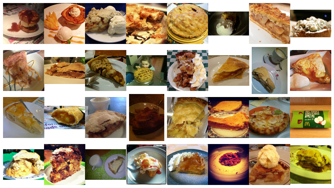
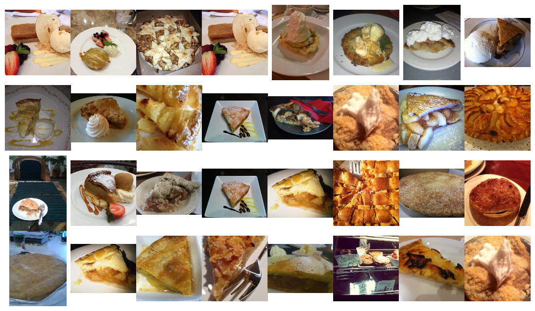
各食品クラスのランダムな画像を見てみましょう。新しいウィンドウで画像を右クリックして開くか、それを保存して、より高い解像度で見ることができます。
 root_dir = 'food-101/images/'
rows = 17
cols = 6
fig , ax = plt . subplots ( rows , cols , frameon = False , figsize = ( 15 , 25 ))
fig . suptitle ( 'Random Image from Each Food Class' , fontsize = 20 )
sorted_food_dirs = sorted ( os . listdir ( root_dir ))
for i in range ( rows ):
    for j in range ( cols ):
        try :
            food_dir = sorted_food_dirs [ i * cols + j ]
        except :
            break
        all_files = os . listdir ( os . path . join ( root_dir , food_dir ))
        rand_img = np . random . choice ( all_files )
        img = plt . imread ( os . path . join ( root_dir , food_dir , rand_img ))
        ax [ i ][ j ]. imshow ( img )
        ec = ( 0 , .6 , .1 )
        fc = ( 0 , .7 , .2 )
        ax [ i ][ j ]. text ( 0 , - 20 , food_dir , size = 10 , rotation = 0 ,
                ha = "left" , va = "top" ,
                bbox = dict ( boxstyle = "round" , ec = ec , fc = fc ))
plt . setp ( ax , xticks = [], yticks = [])
plt . tight_layout ( rect = [ 0 , 0.03 , 1 , 0.95 ])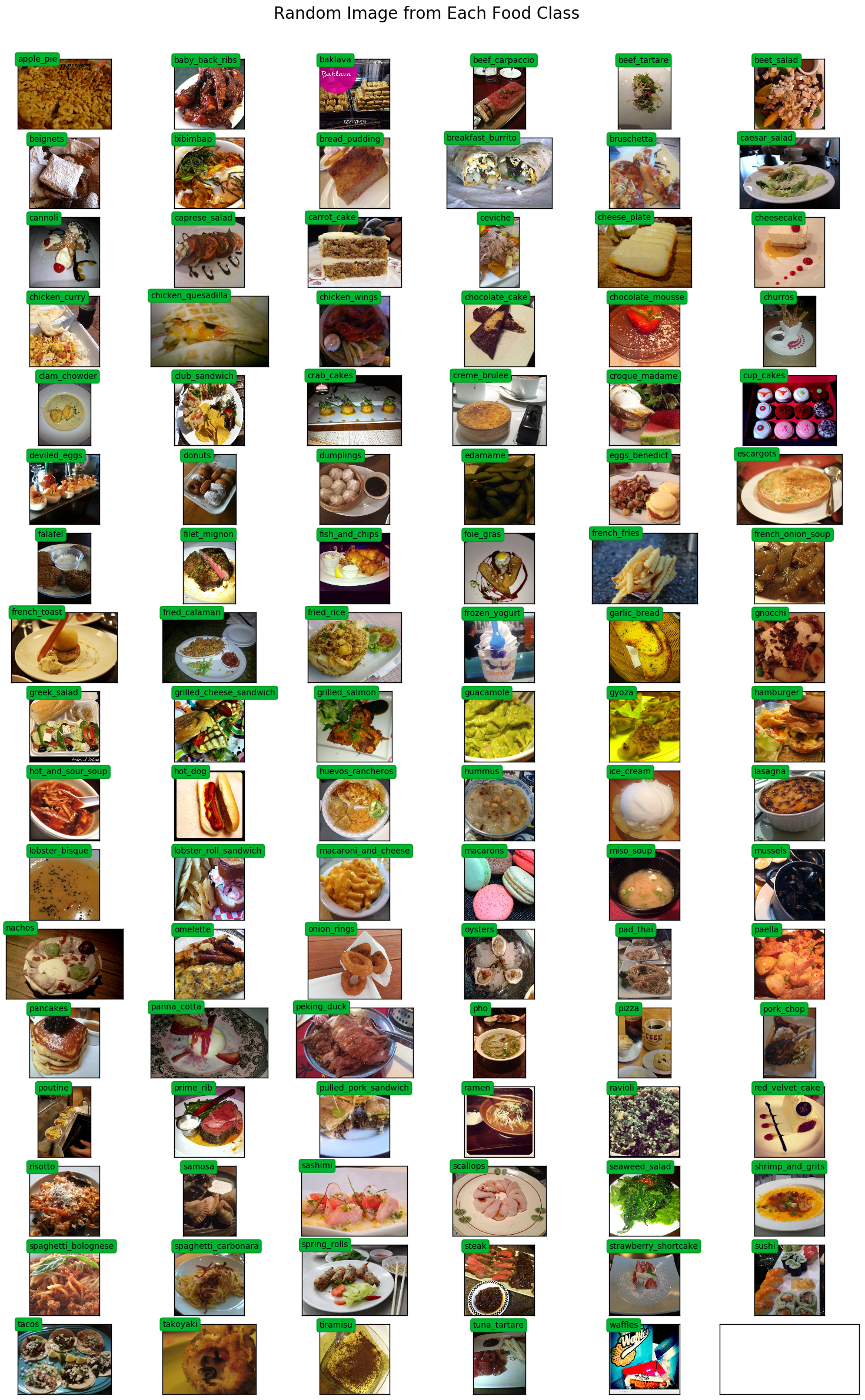
multiprocessing.Poolを使用して、トレーニング中の画像の増強を加速します。
 # Setup multiprocessing pool
# Do this early, as once images are loaded into memory there will be Errno 12
# http://stackoverflow.com/questions/14749897/python-multiprocessing-memory-usage
import multiprocessing as mp

num_processes = 6
pool = mp . Pool ( processes = num_processes )
適切なラベルエンコーディングときれいな印刷のために、クラスからインデックスまでの地図とその逆が必要です。
 class_to_ix = {}
ix_to_class = {}
with open ( 'food-101/meta/classes.txt' , 'r' ) as txt :
    classes = [ l . strip () for l in txt . readlines ()]
    class_to_ix = dict ( zip ( classes , range ( len ( classes ))))
    ix_to_class = dict ( zip ( range ( len ( classes )), classes ))
    class_to_ix = { v : k for k , v in ix_to_class . items ()}
sorted_class_to_ix = collections . OrderedDict ( sorted ( class_to_ix . items ()))
Food-101データセットには、列車/テストの分割が提供されています。分類パフォーマンスを他の実装と比較するために、これを使用したいと考えています。
 # Only split files if haven't already
if not os . path . isdir ( './food-101/test' ) and not os . path . isdir ( './food-101/train' ):

    def copytree ( src , dst , symlinks = False , ignore = None ):
        if not os . path . exists ( dst ):
            os . makedirs ( dst )
            shutil . copystat ( src , dst )
        lst = os . listdir ( src )
        if ignore :
            excl = ignore ( src , lst )
            lst = [ x for x in lst if x not in excl ]
        for item in lst :
            s = os . path . join ( src , item )
            d = os . path . join ( dst , item )
            if symlinks and os . path . islink ( s ):
                if os . path . lexists ( d ):
                    os . remove ( d )
                os . symlink ( os . readlink ( s ), d )
                try :
                    st = os . lstat ( s )
                    mode = stat . S_IMODE ( st . st_mode )
                    os . lchmod ( d , mode )
                except :
                    pass # lchmod not available
            elif os . path . isdir ( s ):
                copytree ( s , d , symlinks , ignore )
            else :
                shutil . copy2 ( s , d )

    def generate_dir_file_map ( path ):
        dir_files = defaultdict ( list )
        with open ( path , 'r' ) as txt :
            files = [ l . strip () for l in txt . readlines ()]
            for f in files :
                dir_name , id = f . split ( '/' )
                dir_files [ dir_name ]. append ( id + '.jpg' )
        return dir_files

    train_dir_files = generate_dir_file_map ( 'food-101/meta/train.txt' )
    test_dir_files = generate_dir_file_map ( 'food-101/meta/test.txt' )


    def ignore_train ( d , filenames ):
        print ( d )
        subdir = d . split ( '/' )[ - 1 ]
        to_ignore = train_dir_files [ subdir ]
        return to_ignore

    def ignore_test ( d , filenames ):
        print ( d )
        subdir = d . split ( '/' )[ - 1 ]
        to_ignore = test_dir_files [ subdir ]
        return to_ignore

    copytree ( 'food-101/images' , 'food-101/test' , ignore = ignore_train )
    copytree ( 'food-101/images' , 'food-101/train' , ignore = ignore_test )

else :
    print ( 'Train/Test files already copied into separate folders.' )
Train/Test files already copied into separate folders.
トレーニングとテスト画像をメモリにロードする準備ができました。すべてがロードされた後、約80 GBのメモリが割り当てられます。
min_sizeよりも小さい幅または長さを持つ画像は、サイズ変更されます。これは、画像の増強中に適切なサイズの作物を摂取できるようにするためです。
 % % time

# Load dataset images and resize to meet minimum width and height pixel size
def load_images ( root , min_side = 299 ):
    all_imgs = []
    all_classes = []
    resize_count = 0
    invalid_count = 0
    for i , subdir in enumerate ( listdir ( root )):
        imgs = listdir ( join ( root , subdir ))
        class_ix = class_to_ix [ subdir ]
        print ( i , class_ix , subdir )
        for img_name in imgs :
            img_arr = img . imread ( join ( root , subdir , img_name ))
            img_arr_rs = img_arr
            try :
                w , h , _ = img_arr . shape
                if w < min_side :
                    wpercent = ( min_side / float ( w ))
                    hsize = int (( float ( h ) * float ( wpercent )))
                    #print('new dims:', min_side, hsize)
                    img_arr_rs = imresize ( img_arr , ( min_side , hsize ))
                    resize_count += 1
                elif h < min_side :
                    hpercent = ( min_side / float ( h ))
                    wsize = int (( float ( w ) * float ( hpercent )))
                    #print('new dims:', wsize, min_side)
                    img_arr_rs = imresize ( img_arr , ( wsize , min_side ))
                    resize_count += 1
                all_imgs . append ( img_arr_rs )
                all_classes . append ( class_ix )
            except :
                print ( 'Skipping bad image: ' , subdir , img_name )
                invalid_count += 1
    print ( len ( all_imgs ), 'images loaded' )
    print ( resize_count , 'images resized' )
    print ( invalid_count , 'images skipped' )
    return np . array ( all_imgs ), np . array ( all_classes )

X_test , y_test = load_images ( 'food-101/test' , min_side = 299 )
0 41 french_onion_soup
1 99 tuna_tartare
2 2 baklava
3 12 cannoli
4 8 bread_pudding
5 58 ice_cream
6 63 macarons
7 38 fish_and_chips
8 3 beef_carpaccio
9 59 lasagna
10 84 risotto
11 53 hamburger
12 7 bibimbap
13 15 ceviche
14 92 spring_rolls
15 78 poutine
16 76 pizza
17 19 chicken_quesadilla
18 71 paella
19 11 caesar_salad
20 30 deviled_eggs
21 40 french_fries
22 25 club_sandwich
23 77 pork_chop
24 31 donuts
25 93 steak
26 43 fried_calamari
27 52 gyoza
28 20 chicken_wings
29 47 gnocchi
30 46 garlic_bread
31 81 ramen
32 86 sashimi
33 100 waffles
34 60 lobster_bisque
35 23 churros
36 1 baby_back_ribs
37 0 apple_pie
38 27 creme_brulee
39 79 prime_rib
40 54 hot_and_sour_soup
41 55 hot_dog
42 82 ravioli
43 66 nachos
44 85 samosa
45 95 sushi
46 70 pad_thai
47 87 scallops
48 42 french_toast
49 13 caprese_salad
50 21 chocolate_cake
51 83 red_velvet_cake
52 88 seaweed_salad
53 96 tacos
54 16 cheesecake
55 90 spaghetti_bolognese
56 94 strawberry_shortcake
57 64 miso_soup
58 98 tiramisu
59 74 peking_duck
60 17 cheese_plate
61 69 oysters
62 14 carrot_cake
63 6 beignets
64 61 lobster_roll_sandwich
65 45 frozen_yogurt
66 24 clam_chowder
67 9 breakfast_burrito
68 72 pancakes
69 32 dumplings
70 57 hummus
71 10 bruschetta
72 44 fried_rice
73 97 takoyaki
74 50 grilled_salmon
75 4 beef_tartare
76 89 shrimp_and_grits
77 28 croque_madame
78 49 grilled_cheese_sandwich
79 80 pulled_pork_sandwich
80 56 huevos_rancheros
81 35 escargots
82 91 spaghetti_carbonara
83 34 eggs_benedict
84 33 edamame
85 22 chocolate_mousse
86 18 chicken_curry
87 65 mussels
88 36 falafel
89 37 filet_mignon
90 26 crab_cakes
91 48 greek_salad
92 5 beet_salad
93 51 guacamole
94 29 cup_cakes
95 68 onion_rings
96 39 foie_gras
97 67 omelette
98 73 panna_cotta
99 75 pho
100 62 macaroni_and_cheese
25250 images loaded
693 images resized
0 images skipped
CPU times: user 1min 18s, sys: 4.82 s, total: 1min 23s
Wall time: 1min 23s
 % % time
X_train , y_train = load_images ( 'food-101/train' , min_side = 299 )
0 41 french_onion_soup
1 99 tuna_tartare
2 2 baklava
3 12 cannoli
4 8 bread_pudding
Skipping bad image: bread_pudding 1375816.jpg
5 58 ice_cream
6 63 macarons
7 38 fish_and_chips
8 3 beef_carpaccio
9 59 lasagna
Skipping bad image: lasagna 3787908.jpg
10 84 risotto
11 53 hamburger
12 7 bibimbap
13 15 ceviche
14 92 spring_rolls
15 78 poutine
16 76 pizza
17 19 chicken_quesadilla
18 71 paella
19 11 caesar_salad
20 30 deviled_eggs
21 40 french_fries
22 25 club_sandwich
23 77 pork_chop
24 31 donuts
25 93 steak
Skipping bad image: steak 1340977.jpg
26 43 fried_calamari
27 52 gyoza
28 20 chicken_wings
29 47 gnocchi
30 46 garlic_bread
31 81 ramen
32 86 sashimi
33 100 waffles
34 60 lobster_bisque
35 23 churros
36 1 baby_back_ribs
37 0 apple_pie
38 27 creme_brulee
39 79 prime_rib
40 54 hot_and_sour_soup
41 55 hot_dog
42 82 ravioli
43 66 nachos
44 85 samosa
45 95 sushi
46 70 pad_thai
47 87 scallops
48 42 french_toast
49 13 caprese_salad
50 21 chocolate_cake
51 83 red_velvet_cake
52 88 seaweed_salad
53 96 tacos
54 16 cheesecake
55 90 spaghetti_bolognese
56 94 strawberry_shortcake
57 64 miso_soup
58 98 tiramisu
59 74 peking_duck
60 17 cheese_plate
61 69 oysters
62 14 carrot_cake
63 6 beignets
64 61 lobster_roll_sandwich
65 45 frozen_yogurt
66 24 clam_chowder
67 9 breakfast_burrito
68 72 pancakes
69 32 dumplings
70 57 hummus
71 10 bruschetta
72 44 fried_rice
73 97 takoyaki
74 50 grilled_salmon
75 4 beef_tartare
76 89 shrimp_and_grits
77 28 croque_madame
78 49 grilled_cheese_sandwich
79 80 pulled_pork_sandwich
80 56 huevos_rancheros
81 35 escargots
82 91 spaghetti_carbonara
83 34 eggs_benedict
84 33 edamame
85 22 chocolate_mousse
86 18 chicken_curry
87 65 mussels
88 36 falafel
89 37 filet_mignon
90 26 crab_cakes
91 48 greek_salad
92 5 beet_salad
93 51 guacamole
94 29 cup_cakes
95 68 onion_rings
96 39 foie_gras
97 67 omelette
98 73 panna_cotta
99 75 pho
100 62 macaroni_and_cheese
75747 images loaded
2091 images resized
3 images skipped
CPU times: user 3min 51s, sys: 13.9 s, total: 4min 5s
Wall time: 4min 5s
 print ( 'X_train shape' , X_train . shape )
print ( 'y_train shape' , y_train . shape )
print ( 'X_test shape' , X_test . shape )
print ( 'y_test shape' , y_test . shape )
X_train shape (75747,)
y_train shape (75747,)
X_test shape (25250,)
y_test shape (25250,)
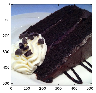
 @ interact ( n = ( 0 , len ( X_train )))
def show_pic ( n ):
    plt . imshow ( X_train [ n ])
    print ( 'class:' , y_train [ n ], ix_to_class [ y_train [ n ]])
class: 21 chocolate_cake
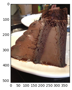
 @ interact ( n = ( 0 , len ( X_test )))
def show_pic ( n ):
    plt . imshow ( X_test [ n ])
    print ( 'class:' , y_test [ n ], ix_to_class [ y_test [ n ]])
class: 21 chocolate_cake
 @ interact ( n_class = sorted_class_to_ix )
def show_random_images_of_class ( n_class = 0 ):
    print ( n_class )
    nrows = 4
    ncols = 8
    fig , axes = plt . subplots ( nrows = nrows , ncols = ncols )
    fig . set_size_inches ( 12 , 8 )
    #fig.tight_layout()
    imgs = np . random . choice (( y_train == n_class ). nonzero ()[ 0 ], nrows * ncols )
    for i , ax in enumerate ( axes . flat ):
        im = ax . imshow ( X_train [ imgs [ i ]])
        ax . set_axis_off ()
        ax . title . set_visible ( False )
        ax . xaxis . set_ticks ([])
        ax . yaxis . set_ticks ([])
        for spine in ax . spines . values ():
            spine . set_visible ( False )
    plt . subplots_adjust ( left = 0 , wspace = 0 , hspace = 0 )
    plt . show ()
0
 @ interact ( n_class = sorted_class_to_ix )
def show_random_images_of_class ( n_class = 0 ):
    print ( n_class )
    nrows = 4
    ncols = 8
    fig , axes = plt . subplots ( nrows = nrows , ncols = ncols )
    fig . set_size_inches ( 12 , 8 )
    #fig.tight_layout()
    imgs = np . random . choice (( y_test == n_class ). nonzero ()[ 0 ], nrows * ncols )
    for i , ax in enumerate ( axes . flat ):
        im = ax . imshow ( X_test [ imgs [ i ]])
        ax . set_axis_off ()
        ax . title . set_visible ( False )
        ax . xaxis . set_ticks ([])
        ax . yaxis . set_ticks ([])
        for spine in ax . spines . values ():
            spine . set_visible ( False )
    plt . subplots_adjust ( left = 0 , wspace = 0 , hspace = 0 )
    plt . show ()
0
n_classes値を使用できる1つの機能ではなく、バイナリ機能のベクトルを作成するには、各ラベル値を1ホットにエンコードする必要があります。
 from keras . utils . np_utils import to_categorical

n_classes = 101
y_train_cat = to_categorical ( y_train , nb_classes = n_classes )
y_test_cat = to_categorical ( y_test , nb_classes = n_classes )
from keras . applications . inception_v3 import InceptionV3
from keras . applications . inception_v3 import preprocess_input , decode_predictions
from keras . preprocessing import image
from keras . layers import Input
import tools . image_gen_extended as T
# Useful for checking the output of the generators after code change
#from importlib import reload
#reload(T)ケラスに出荷するものよりも、より強力な画像増強パイプラインが必要でした。幸いなことに、私は自分のベースとして使用するこの変更されたバージョンを見つけることができました。
著者は、拡張可能なパイプラインを追加していたため、カスタムクロッピング機能やInception Image Preprocessorの使用などの追加の変更を指定できました。すべてのトレーニングセットをfloat32sとして保持するのに十分なメモリがなかったため、前処理を動的に適用できることが必要でした。トレーニングセット全体をuint8sとしてロードすることができました。
さらに、GPUまたはマルチコアCPUのいずれを完全に活用していませんでした。デフォルトでは、Pythonは単一のコアのみを使用できるため、トレーニングのためにGPUに送信できる処理/拡張画像の量が制限されます。いくつかのパフォーマンス監視に基づいて、私は平均してGPUのわずかな割合しか使用していませんでした。 Python multiprocessing Poolを組み込むことで、約50%のCPU使用率と90%のGPU使用率を取得することができました。
最終結果は、トレーニングの各エポックが45分から22分になったことです!このノートブックでトレーニング中にGPUグラフを実行できます。データ増強とGPUパフォーマンスを改善しようとするためのインスピレーションは、Jimmie Goode:データ増強のためのバッファリングされたPythonジェネレーターから来ました
現時点では、コードはかなりバギーで、トレーニングが手動で中断されるたびにPythonカーネルを再起動する必要があります。コードは非常にハッキングされており、フィッティングを伴う機能のような特定の機能は無効です。このイメージガネレーターを改善し、将来コミュニティにリリースしたいと考えています。
display ( Image ( './gpu.png' ))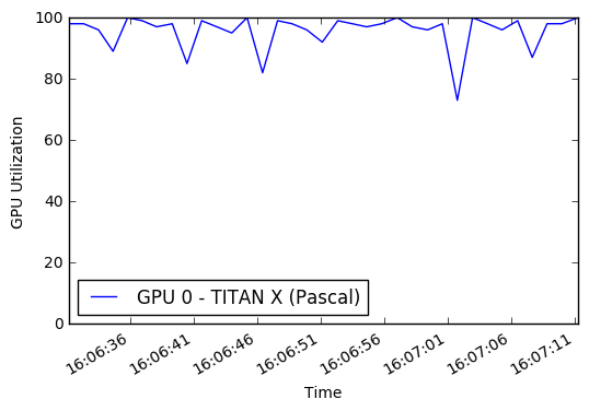
 % % time

# this is the augmentation configuration we will use for training
train_datagen = T . ImageDataGenerator (
    featurewise_center = False ,  # set input mean to 0 over the dataset
    samplewise_center = False ,  # set each sample mean to 0
    featurewise_std_normalization = False ,  # divide inputs by std of the dataset
    samplewise_std_normalization = False ,  # divide each input by its std
    zca_whitening = False ,  # apply ZCA whitening
    rotation_range = 0 ,  # randomly rotate images in the range (degrees, 0 to 180)
    width_shift_range = 0.2 ,  # randomly shift images horizontally (fraction of total width)
    height_shift_range = 0.2 ,  # randomly shift images vertically (fraction of total height)
    horizontal_flip = True ,  # randomly flip images
    vertical_flip = False , # randomly flip images
    zoom_range = [ .8 , 1 ],
    channel_shift_range = 30 ,
    fill_mode = 'reflect' )
train_datagen . config [ 'random_crop_size' ] = ( 299 , 299 )
train_datagen . set_pipeline ([ T . random_transform , T . random_crop , T . preprocess_input ])
train_generator = train_datagen . flow ( X_train , y_train_cat , batch_size = 64 , seed = 11 , pool = pool )
test_datagen = T . ImageDataGenerator ()
test_datagen . config [ 'random_crop_size' ] = ( 299 , 299 )
test_datagen . set_pipeline ([ T . random_transform , T . random_crop , T . preprocess_input ])
test_generator = test_datagen . flow ( X_test , y_test_cat , batch_size = 64 , seed = 11 , pool = pool )これらのイメージガネレーターからどのような画像が出ているかを見ることができます。
 def reverse_preprocess_input ( x0 ):
    x = x0 / 2.0
    x += 0.5
    x *= 255.
    return x
% % time
@ interact ()
def show_images ( unprocess = True ):
for x in test_generator :
fig , axes = plt . subplots ( nrows = 8 , ncols = 4 )
fig . set_size_inches ( 8 , 8 )
page = 0
page_size = 32
start_i = page * page_size
for i , ax in enumerate ( axes . flat ):
img = x [ 0 ][ i + start_i ]
if unprocess :
im = ax . imshow ( reverse_preprocess_input ( img ). astype ( 'uint8' ) )
else :
im = ax . imshow ( img )
ax . set_axis_off ()
ax . title . set_visible ( False )
ax . xaxis . set_ticks ([])
ax . yaxis . set_ticks ([])
for spine in ax . spines . values ():
spine . set_visible ( False )
plt . subplots_adjust ( left = 0 , wspace = 0 , hspace = 0 )
plt . show ()
break 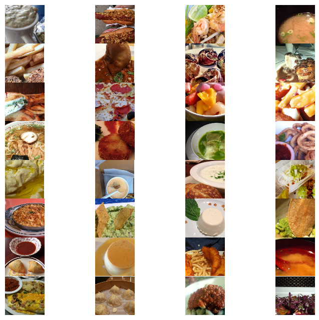
 CPU times: user 1.54 s, sys: 524 ms, total: 2.06 s
Wall time: 2.24 s
 % % time
show_images ( unprocess = False )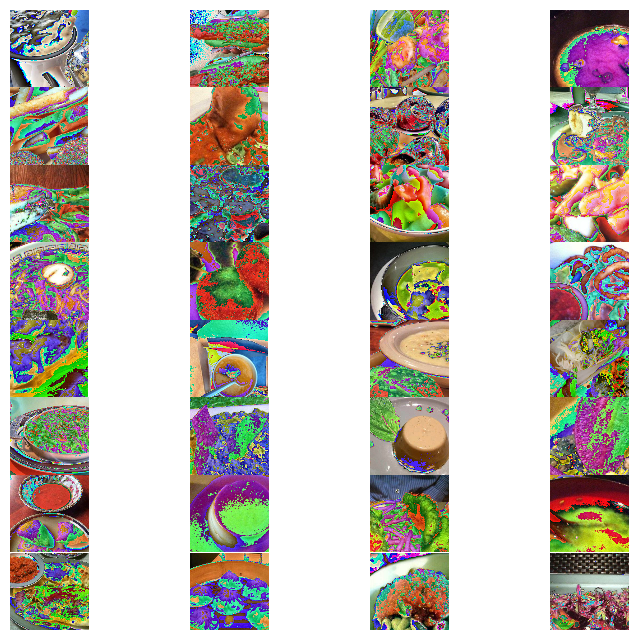
 CPU times: user 1.58 s, sys: 300 ms, total: 1.88 s
Wall time: 2.11 s
Imagenetで前提としたGoogle InceptionV3モデルを再訓練します。ニューラルネットワークアーキテクチャを以下に示します。
 % % time
from keras . models import Sequential , Model
from keras . layers import Dense , Dropout , Activation , Flatten
from keras . layers import Convolution2D , MaxPooling2D , ZeroPadding2D , GlobalAveragePooling2D , AveragePooling2D
from keras . layers . normalization import BatchNormalization
from keras . preprocessing . image import ImageDataGenerator
from keras . callbacks import ModelCheckpoint , CSVLogger , LearningRateScheduler , ReduceLROnPlateau
from keras . optimizers import SGD
from keras . regularizers import l2
import keras . backend as K
import math

K . clear_session ()

base_model = InceptionV3 ( weights = 'imagenet' , include_top = False , input_tensor = Input ( shape = ( 299 , 299 , 3 )))
x = base_model . output
x = AveragePooling2D ( pool_size = ( 8 , 8 ))( x )
x = Dropout ( .4 )( x )
x = Flatten ()( x )
predictions = Dense ( n_classes , init = 'glorot_uniform' , W_regularizer = l2 ( .0005 ), activation = 'softmax' )( x )

model = Model ( input = base_model . input , output = predictions )

opt = SGD ( lr = .01 , momentum = .9 )
model . compile ( optimizer = opt , loss = 'categorical_crossentropy' , metrics = [ 'accuracy' ])

checkpointer = ModelCheckpoint ( filepath = 'model4.{epoch:02d}-{val_loss:.2f}.hdf5' , verbose = 1 , save_best_only = True )
csv_logger = CSVLogger ( 'model4.log' )

def schedule ( epoch ):
    if epoch < 15 :
        return .01
    elif epoch < 28 :
        return .002
    else :
        return .0004
lr_scheduler = LearningRateScheduler ( schedule )

model . fit_generator ( train_generator ,
                    validation_data = test_generator ,
                    nb_val_samples = X_test . shape [ 0 ],
                    samples_per_epoch = X_train . shape [ 0 ],
                    nb_epoch = 32 ,
                    verbose = 2 ,
                    callbacks = [ lr_scheduler , csv_logger , checkpointer ])
Epoch 1/32
Epoch 00000: val_loss improved from inf to 3.37355, saving model to model4.00-3.37.hdf5
1342s - loss: 4.2541 - acc: 0.0810 - val_loss: 3.3736 - val_acc: 0.2010
Epoch 2/32
Epoch 00001: val_loss improved from 3.37355 to 2.36625, saving model to model4.01-2.37.hdf5
1329s - loss: 2.9745 - acc: 0.3075 - val_loss: 2.3662 - val_acc: 0.4071
Epoch 3/32
Epoch 00002: val_loss improved from 2.36625 to 1.79355, saving model to model4.02-1.79.hdf5
1329s - loss: 2.3080 - acc: 0.4539 - val_loss: 1.7935 - val_acc: 0.5338
Epoch 4/32
Epoch 00003: val_loss improved from 1.79355 to 1.48898, saving model to model4.03-1.49.hdf5
1356s - loss: 2.0102 - acc: 0.5216 - val_loss: 1.4890 - val_acc: 0.6068
Epoch 5/32
Epoch 00004: val_loss improved from 1.48898 to 1.34121, saving model to model4.04-1.34.hdf5
1330s - loss: 1.8436 - acc: 0.5577 - val_loss: 1.3412 - val_acc: 0.6431
Epoch 6/32
Epoch 00005: val_loss improved from 1.34121 to 1.22485, saving model to model4.05-1.22.hdf5
1329s - loss: 1.7057 - acc: 0.5909 - val_loss: 1.2248 - val_acc: 0.6740
Epoch 7/32
Epoch 00006: val_loss did not improve
1328s - loss: 1.5996 - acc: 0.6126 - val_loss: 1.2310 - val_acc: 0.6716
Epoch 8/32
Epoch 00007: val_loss improved from 1.22485 to 1.11248, saving model to model4.07-1.11.hdf5
1331s - loss: 1.5148 - acc: 0.6314 - val_loss: 1.1125 - val_acc: 0.7022
Epoch 9/32
Epoch 00008: val_loss improved from 1.11248 to 1.07145, saving model to model4.08-1.07.hdf5
1331s - loss: 1.4395 - acc: 0.6506 - val_loss: 1.0714 - val_acc: 0.7095
Epoch 10/32
Epoch 00009: val_loss improved from 1.07145 to 1.05129, saving model to model4.09-1.05.hdf5
1333s - loss: 1.3900 - acc: 0.6637 - val_loss: 1.0513 - val_acc: 0.7181
Epoch 11/32
Epoch 00010: val_loss improved from 1.05129 to 1.03356, saving model to model4.10-1.03.hdf5
1331s - loss: 1.3316 - acc: 0.6780 - val_loss: 1.0336 - val_acc: 0.7250
Epoch 12/32
Epoch 00011: val_loss improved from 1.03356 to 1.00622, saving model to model4.11-1.01.hdf5
1331s - loss: 1.2850 - acc: 0.6893 - val_loss: 1.0062 - val_acc: 0.7275
Epoch 13/32
Epoch 00012: val_loss improved from 1.00622 to 0.94016, saving model to model4.12-0.94.hdf5
1330s - loss: 1.2325 - acc: 0.7003 - val_loss: 0.9402 - val_acc: 0.7461
Epoch 14/32
Epoch 00013: val_loss did not improve
1330s - loss: 1.1970 - acc: 0.7086 - val_loss: 0.9461 - val_acc: 0.7453
Epoch 15/32
Epoch 00014: val_loss did not improve
1329s - loss: 1.1683 - acc: 0.7154 - val_loss: 0.9691 - val_acc: 0.7396
Epoch 16/32
Epoch 00015: val_loss improved from 0.94016 to 0.71776, saving model to model4.15-0.72.hdf5
1329s - loss: 0.9398 - acc: 0.7724 - val_loss: 0.7178 - val_acc: 0.8055
Epoch 17/32
Epoch 00016: val_loss improved from 0.71776 to 0.70245, saving model to model4.16-0.70.hdf5
1329s - loss: 0.8591 - acc: 0.7916 - val_loss: 0.7025 - val_acc: 0.8069
Epoch 18/32
Epoch 00017: val_loss did not improve
1327s - loss: 0.8238 - acc: 0.8023 - val_loss: 0.7093 - val_acc: 0.8053
Epoch 19/32
Epoch 00018: val_loss did not improve
1327s - loss: 0.7947 - acc: 0.8093 - val_loss: 0.7048 - val_acc: 0.8059
Epoch 20/32
Epoch 00019: val_loss did not improve
1327s - loss: 0.7713 - acc: 0.8143 - val_loss: 0.7097 - val_acc: 0.8061
Epoch 21/32
Epoch 00020: val_loss improved from 0.70245 to 0.69545, saving model to model4.20-0.70.hdf5
1329s - loss: 0.7458 - acc: 0.8195 - val_loss: 0.6955 - val_acc: 0.8104
Epoch 22/32
Epoch 00021: val_loss did not improve
1328s - loss: 0.7282 - acc: 0.8232 - val_loss: 0.6977 - val_acc: 0.8119
Epoch 23/32
Epoch 00022: val_loss improved from 0.69545 to 0.69190, saving model to model4.22-0.69.hdf5
1328s - loss: 0.7114 - acc: 0.8284 - val_loss: 0.6919 - val_acc: 0.8150
Epoch 24/32
Epoch 00023: val_loss did not improve
1325s - loss: 0.6983 - acc: 0.8311 - val_loss: 0.7002 - val_acc: 0.8116
Epoch 25/32
Epoch 00024: val_loss did not improve
1330s - loss: 0.6719 - acc: 0.8381 - val_loss: 0.7031 - val_acc: 0.8112
Epoch 26/32
Epoch 00025: val_loss did not improve
1382s - loss: 0.6607 - acc: 0.8407 - val_loss: 0.7115 - val_acc: 0.8083
Epoch 27/32
Epoch 00026: val_loss did not improve
1330s - loss: 0.6479 - acc: 0.8439 - val_loss: 0.7037 - val_acc: 0.8126
Epoch 28/32
Epoch 00027: val_loss did not improve
1328s - loss: 0.6292 - acc: 0.8478 - val_loss: 0.7122 - val_acc: 0.8086
Epoch 29/32
Epoch 00028: val_loss improved from 0.69190 to 0.68908, saving model to model4.28-0.69.hdf5
1330s - loss: 0.5983 - acc: 0.8580 - val_loss: 0.6891 - val_acc: 0.8165
Epoch 30/32
Epoch 00029: val_loss improved from 0.68908 to 0.68740, saving model to model4.29-0.69.hdf5
1330s - loss: 0.5817 - acc: 0.8612 - val_loss: 0.6874 - val_acc: 0.8149
Epoch 31/32
Epoch 00030: val_loss did not improve
1328s - loss: 0.5729 - acc: 0.8642 - val_loss: 0.6912 - val_acc: 0.8143
Epoch 32/32
Epoch 00031: val_loss did not improve
1329s - loss: 0.5638 - acc: 0.8663 - val_loss: 0.6895 - val_acc: 0.8159
CPU times: user 8h 49min 20s, sys: 1h 55min 54s, total: 10h 45min 14s
Wall time: 11h 51min 18s
この時点で、テストセットで最大81.65のシングルクロップトップ1の精度が見られます。さらに遅い学習率でモデルをトレーニングし続けることができ、それがさらに改善されるかどうかを確認できます。
私の最初の実験では、高等教育率とともに、AdamやAdadeltaなどのより近代的なオプティマザーを使用しました。文献をより密接に従うことにし、学習スケジュールを迅速に減少させて確率勾配降下(SGD)を使用することを決定する前に、私はしばらく80%未満の精度を下回っていました。多次元表面を検索しているとき、時々遅くなることは長い道のりを歩むことがあります。
マルチプロセッシングコードにはある程度の不安定性があるため、ノートブックを再起動し、最新モデルをロードしてからトレーニングを続ける必要がある場合があります。
 % % time
from keras . models import Sequential , Model , load_model
from keras . layers import Dense , Dropout , Activation , Flatten
from keras . layers import Convolution2D , MaxPooling2D , ZeroPadding2D , GlobalAveragePooling2D , AveragePooling2D
from keras . layers . normalization import BatchNormalization
from keras . preprocessing . image import ImageDataGenerator
from keras . callbacks import ModelCheckpoint , CSVLogger , LearningRateScheduler , ReduceLROnPlateau
from keras . optimizers import SGD
from keras . regularizers import l2
import keras . backend as K
import math

model = load_model ( filepath = './model4.29-0.69.hdf5' )

opt = SGD ( lr = .01 , momentum = .9 )
model . compile ( optimizer = opt , loss = 'categorical_crossentropy' , metrics = [ 'accuracy' ])

checkpointer = ModelCheckpoint ( filepath = 'model4b.{epoch:02d}-{val_loss:.2f}.hdf5' , verbose = 1 , save_best_only = True )
csv_logger = CSVLogger ( 'model4b.log' )

def schedule ( epoch ):
    if epoch < 10 :
        return .00008
    elif epoch < 20 :
        return .000016
    else :
        return .0000032

lr_scheduler = LearningRateScheduler ( schedule )

model . fit_generator ( train_generator ,
                    validation_data = test_generator ,
                    nb_val_samples = X_test . shape [ 0 ],
                    samples_per_epoch = X_train . shape [ 0 ],
                    nb_epoch = 32 ,
                    verbose = 2 ,
callbacks = [ lr_scheduler , csv_logger , checkpointer ])この時点で、複数のトレーニングモデルをディスクに保存する必要があります。それらを通過し、 load_model関数を使用して、モデルを最低の損失 /最高精度でロードできます。
 % % time
#model = load_model(filepath='./model4.29-0.69.hdf5') # 86.8039 10-crop Top-1 test accuracy
model = load_model ( filepath = './model4b.10-0.68.hdf5' ) # 86.9703
CPU times: user 36.4 s, sys: 1.11 s, total: 37.5 s
Wall time: 36.5 s
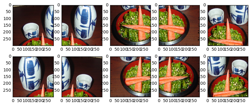
また、複数の作物を使用してテストセットを評価したいと考えています。これにより、単一の作物評価と比較して5%の精度が得られる可能性があります。次の作物を使用するのが一般的です:左上、右上、左下、右下、中央。また、左から右にひっくり返った画像上の同じ作物を取り、合計10個の作物を作成します。
さらに、たとえばトップ5の精度を計算するために、各作物のTOP-N予測を返したいと考えています。
 def center_crop ( x , center_crop_size , ** kwargs ):
    centerw , centerh = x . shape [ 0 ] // 2 , x . shape [ 1 ] // 2
    halfw , halfh = center_crop_size [ 0 ] // 2 , center_crop_size [ 1 ] // 2
    return x [ centerw - halfw : centerw + halfw + 1 , centerh - halfh : centerh + halfh + 1 , :]
def predict_10_crop ( img , ix , top_n = 5 , plot = False , preprocess = True , debug = False ):
flipped_X = np . fliplr ( img )
crops = [
img [: 299 ,: 299 , :], # Upper Left
img [: 299 , img . shape [ 1 ] - 299 :, :], # Upper Right
img [ img . shape [ 0 ] - 299 :, : 299 , :], # Lower Left
img [ img . shape [ 0 ] - 299 :, img . shape [ 1 ] - 299 :, :], # Lower Right
center_crop ( img , ( 299 , 299 )),
flipped_X [: 299 ,: 299 , :],
flipped_X [: 299 , flipped_X . shape [ 1 ] - 299 :, :],
flipped_X [ flipped_X . shape [ 0 ] - 299 :, : 299 , :],
flipped_X [ flipped_X . shape [ 0 ] - 299 :, flipped_X . shape [ 1 ] - 299 :, :],
center_crop ( flipped_X , ( 299 , 299 ))
]
if preprocess :
crops = [ preprocess_input ( x . astype ( 'float32' )) for x in crops ]
if plot :
fig , ax = plt . subplots ( 2 , 5 , figsize = ( 10 , 4 ))
ax [ 0 ][ 0 ]. imshow ( crops [ 0 ])
ax [ 0 ][ 1 ]. imshow ( crops [ 1 ])
ax [ 0 ][ 2 ]. imshow ( crops [ 2 ])
ax [ 0 ][ 3 ]. imshow ( crops [ 3 ])
ax [ 0 ][ 4 ]. imshow ( crops [ 4 ])
ax [ 1 ][ 0 ]. imshow ( crops [ 5 ])
ax [ 1 ][ 1 ]. imshow ( crops [ 6 ])
ax [ 1 ][ 2 ]. imshow ( crops [ 7 ])
ax [ 1 ][ 3 ]. imshow ( crops [ 8 ])
ax [ 1 ][ 4 ]. imshow ( crops [ 9 ])
y_pred = model . predict ( np . array ( crops ))
preds = np . argmax ( y_pred , axis = 1 )
top_n_preds = np . argpartition ( y_pred , - top_n )[:, - top_n :]
if debug :
print ( 'Top-1 Predicted:' , preds )
print ( 'Top-5 Predicted:' , top_n_preds )
print ( 'True Label:' , y_test [ ix ])
return preds , top_n_preds
ix = 13001
predict_10_crop ( X_test [ ix ], ix , top_n = 5 , plot = True , preprocess = False , debug = True ) Top-1 Predicted: [74 74 74 74 74 74 74 74 74 74]
Top-5 Predicted: [[33 97 37 39 74]
[28 52 37 39 74]
[73 39 52 37 74]
[35 33 37 39 74]
[35 33 37 39 74]
[35 33 37 39 74]
[35 33 37 39 74]
[97 37 73 39 74]
[73 52 37 39 74]
[34 35 33 39 74]]
True Label: 88
(array([74, 74, 74, 74, 74, 74, 74, 74, 74, 74]), array([[33, 97, 37, 39, 74],
[28, 52, 37, 39, 74],
[73, 39, 52, 37, 74],
[35, 33, 37, 39, 74],
[35, 33, 37, 39, 74],
[35, 33, 37, 39, 74],
[35, 33, 37, 39, 74],
[97, 37, 73, 39, 74],
[73, 52, 37, 39, 74],
[34, 35, 33, 39, 74]]))
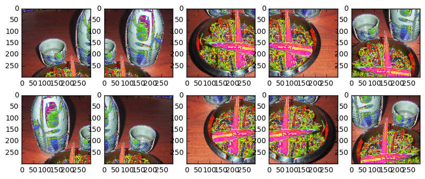
また、Inceptionモデルの画像を前処理する必要があります。
 ix = 13001
predict_10_crop ( X_test [ ix ], ix , top_n = 5 , plot = True , preprocess = True , debug = True )
Top-1 Predicted: [51 51 88 88 88 51 51 88 88 88]
Top-5 Predicted: [[18 79 51 13 48]
[48 79 11 55 51]
[79 93 81 37 88]
[51 86 93 81 88]
[11 79 51 81 88]
[19 79 51 56 13]
[11 88 48 51 13]
[37 93 86 88 81]
[37 79 93 88 81]
[84 81 11 79 88]]
True Label: 88
(array([51, 51, 88, 88, 88, 51, 51, 88, 88, 88]), array([[18, 79, 51, 13, 48],
[48, 79, 11, 55, 51],
[79, 93, 81, 37, 88],
[51, 86, 93, 81, 88],
[11, 79, 51, 81, 88],
[19, 79, 51, 56, 13],
[11, 88, 48, 51, 13],
[37, 93, 86, 88, 81],
[37, 79, 93, 88, 81],
[84, 81, 11, 79, 88]]))
次に、テストセット内の各アイテムの作物を作成し、予測を取得します。私はマルチプロセッシングや他のタイプの並列性を利用していないため、これは現時点で遅いプロセスです。
 % % time
preds_10_crop = {}
for ix in range ( len ( X_test )):
    if ix % 1000 == 0 :
        print ( ix )
    preds_10_crop [ ix ] = predict_10_crop ( X_test [ ix ], ix )
0
1000
2000
3000
4000
5000
6000
7000
8000
9000
10000
11000
12000
13000
14000
15000
16000
17000
18000
19000
20000
21000
22000
23000
24000
25000
CPU times: user 50min 3s, sys: 5min 13s, total: 55min 16s
Wall time: 31min 28s
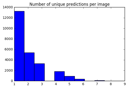
これで、各画像に対して10の予測セットがあります。ヒストグラムを使用して、各画像の一意の予測の#がどのように分散されているかを確認できます。
 preds_uniq = { k : np . unique ( v [ 0 ]) for k , v in preds_10_crop . items ()}
preds_hist = np . array ([ len ( x ) for x in preds_uniq . values ()])

plt . hist ( preds_hist , bins = 11 )
plt . title ( 'Number of unique predictions per image' )
<matplotlib.text.Text at 0x7fe30c3daa20>
テスト項目インデックスをTOP-1 / TOP-5予測にマップする辞書を作成しましょう。
 preds_top_1 = { k : collections . Counter ( v [ 0 ]). most_common ( 1 ) for k , v in preds_10_crop . items ()}

top_5_per_ix = { k : collections . Counter ( preds_10_crop [ k ][ 1 ]. reshape ( - 1 )). most_common ( 5 )
                for k , v in preds_10_crop . items ()}
preds_top_5 = { k : [ y [ 0 ] for y in v ] for k , v in top_5_per_ix . items ()}
% % time
right_counter = 0
for i in range ( len ( y_test )):
guess , actual = preds_top_1 [ i ][ 0 ][ 0 ], y_test [ i ]
if guess == actual :
right_counter += 1
print ( 'Top-1 Accuracy, 10-Crop: {0:.2f}%' . format ( right_counter / len ( y_test ) * 100 )) Top-1 Accuracy, 10-Crop: 86.97%
CPU times: user 28 ms, sys: 0 ns, total: 28 ms
Wall time: 27.3 ms
 % % time
top_5_counter = 0
for i in range ( len ( y_test )):
    guesses , actual = preds_top_5 [ i ], y_test [ i ]
    if actual in guesses :
        top_5_counter += 1

print ( 'Top-5 Accuracy, 10-Crop: {0:.2f}%' . format ( top_5_counter / len ( y_test ) * 100 ))
Top-5 Accuracy, 10-Crop: 97.42%
CPU times: user 28 ms, sys: 0 ns, total: 28 ms
Wall time: 27 ms
y_pred = [ x [ 0 ][ 0 ] for x in preds_top_1 . values ()] @ interact ( page = [ 0 , int ( len ( X_test ) / 20 )])
def show_images_prediction ( page = 0 ):
page_size = 20
nrows = 4
ncols = 5
fig , axes = plt . subplots ( nrows = nrows , ncols = ncols , figsize = ( 12 , 12 ))
fig . set_size_inches ( 12 , 8 )
#fig.tight_layout()
#imgs = np.random.choice((y_all == n_class).nonzero()[0], nrows * ncols)
start_i = page * page_size
for i , ax in enumerate ( axes . flat ):
im = ax . imshow ( X_test [ i + start_i ])
ax . set_axis_off ()
ax . title . set_visible ( False )
ax . xaxis . set_ticks ([])
ax . yaxis . set_ticks ([])
for spine in ax . spines . values ():
spine . set_visible ( False )
predicted = ix_to_class [ y_pred [ i + start_i ]]
match = predicted == ix_to_class [ y_test [ start_i + i ]]
ec = ( 1 , .5 , .5 )
fc = ( 1 , .8 , .8 )
if match :
ec = ( 0 , .6 , .1 )
fc = ( 0 , .7 , .2 )
# predicted label
ax . text ( 0 , 400 , 'P: ' + predicted , size = 10 , rotation = 0 ,
ha = "left" , va = "top" ,
bbox = dict ( boxstyle = "round" ,
ec = ec ,
fc = fc ,
)
)
if not match :
# true label
ax . text ( 0 , 480 , 'A: ' + ix_to_class [ y_test [ start_i + i ]], size = 10 , rotation = 0 ,
ha = "left" , va = "top" ,
bbox = dict ( boxstyle = "round" ,
ec = ec ,
fc = fc ,
)
)
plt . subplots_adjust ( left = 0 , wspace = 1 , hspace = 0 )
plt . show ()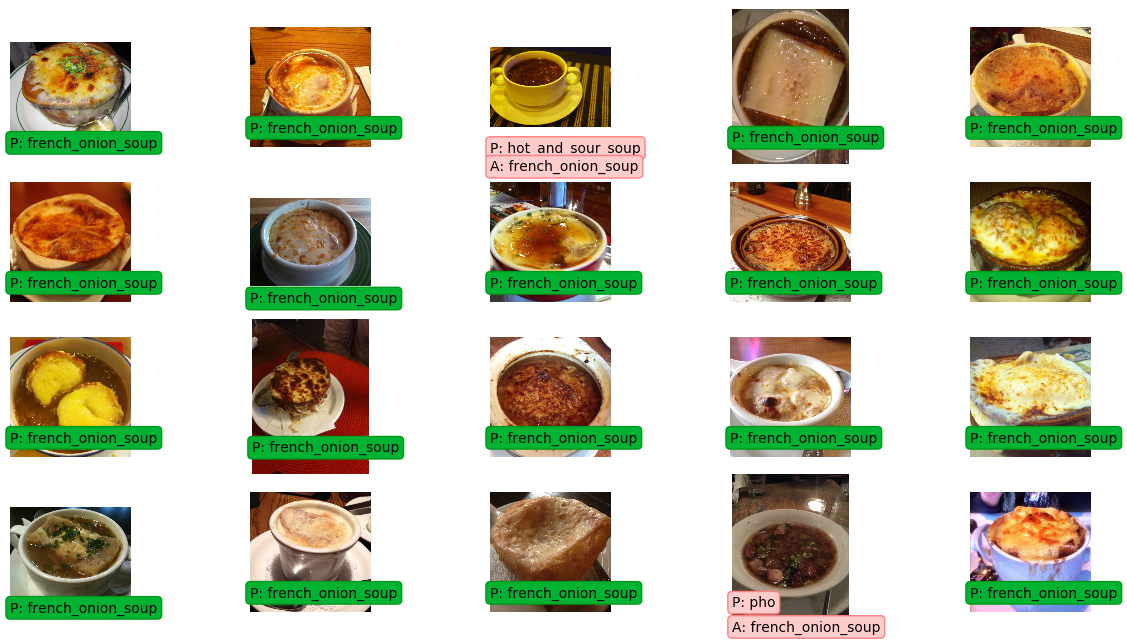
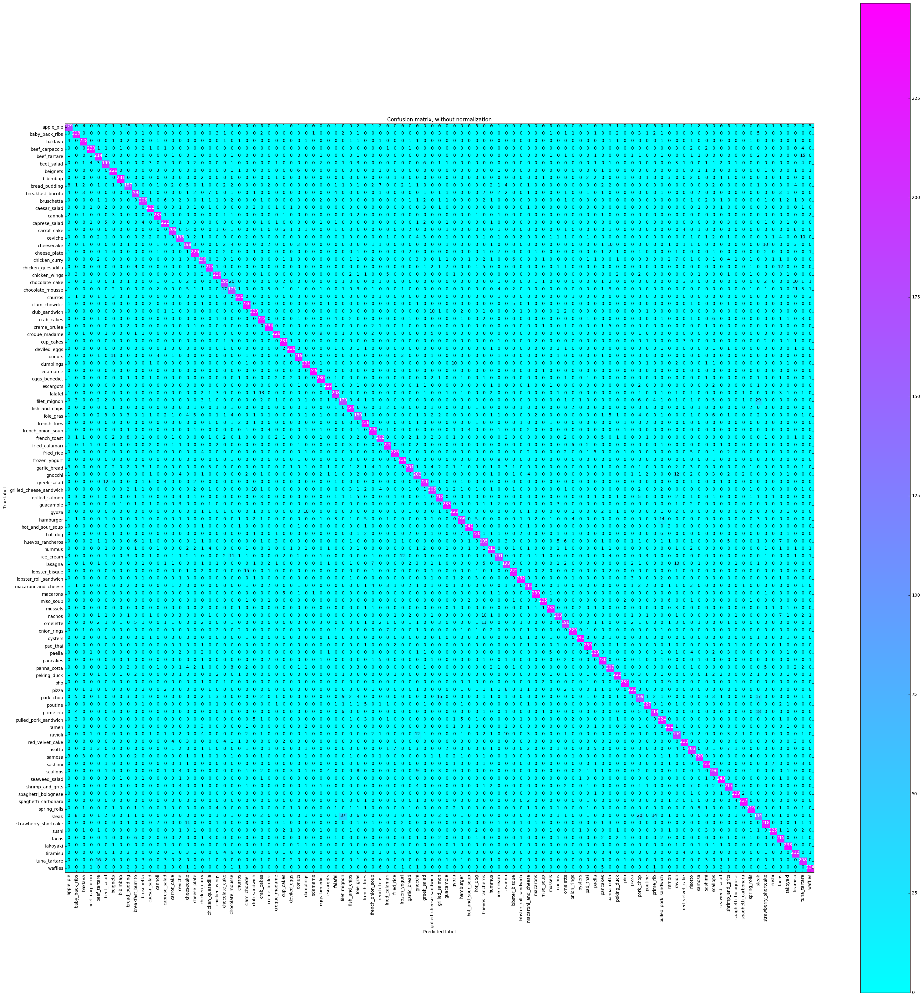
混乱マトリックスは、各クラスのラベルをプロットし、それが正しくラベル付けされた回数と、別のクラスとして誤ってラベル付けされたこともあります。
 % % time
from sklearn . metrics import confusion_matrix
import itertools

def plot_confusion_matrix ( cm , classes ,
                          normalize = False ,
                          title = 'Confusion matrix' ,
                          cmap = plt . cm . Blues ):
    """
    This function prints and plots the confusion matrix.
    Normalization can be applied by setting `normalize=True`.
    """
    plt . imshow ( cm , interpolation = 'nearest' , cmap = cmap )
    plt . title ( title )
    plt . colorbar ()
    tick_marks = np . arange ( len ( classes ))
    plt . xticks ( tick_marks , classes , rotation = 90 )
    plt . yticks ( tick_marks , classes )

    if normalize :
        cm = cm . astype ( 'float' ) / cm . sum ( axis = 1 )[:, np . newaxis ]
        print ( "Normalized confusion matrix" )
    else :
        print ( 'Confusion matrix, without normalization' )

    print ( cm )

    thresh = cm . max () / 2.
    for i , j in itertools . product ( range ( cm . shape [ 0 ]), range ( cm . shape [ 1 ])):
        plt . text ( j , i , cm [ i , j ],
                 horizontalalignment = "center" ,
                 color = "white" if cm [ i , j ] > thresh else "black" )

    plt . tight_layout ()
    plt . ylabel ( 'True label' )
    plt . xlabel ( 'Predicted label' )


# Compute confusion matrix
cnf_matrix = confusion_matrix ( y_test , y_pred )
np . set_printoptions ( precision = 2 )

class_names = [ ix_to_class [ i ] for i in range ( 101 )]

plt . figure ()
fig = plt . gcf ()
fig . set_size_inches ( 32 , 32 )
plot_confusion_matrix ( cnf_matrix , classes = class_names ,
                      title = 'Confusion matrix, without normalization' ,
                      cmap = plt . cm . cool )
plt . show ()
Confusion matrix, without normalization
[[179 0 4 ..., 2 0 5]
[ 0 218 0 ..., 0 0 0]
[ 4 0 228 ..., 1 0 0]
...,
[ 0 0 0 ..., 212 0 1]
[ 0 0 0 ..., 0 208 0]
[ 0 0 0 ..., 0 0 224]]
 CPU times: user 16.4 s, sys: 1.22 s, total: 17.6 s
Wall time: 16.4 s
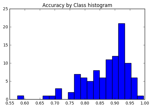
すべてのクラスで精度が一貫しているかどうか、または一部のクラスが他のクラスよりもはるかに簡単 /ラベルを付けるのが難しいかどうかを確認したいと考えています。私たちのプロットによると、いくつかのクラスは、正しくラベルを付けるのがはるかに難しいという点で外れ値でした。
 corrects = collections . defaultdict ( int )
incorrects = collections . defaultdict ( int )
for ( pred , actual ) in zip ( y_pred , y_test ):
    if pred == actual :
        corrects [ actual ] += 1
    else :
        incorrects [ actual ] += 1

class_accuracies = {}
for ix in range ( 101 ):
    class_accuracies [ ix ] = corrects [ ix ] / 250

plt . hist ( list ( class_accuracies . values ()), bins = 20 )
plt . title ( 'Accuracy by Class histogram' )
<matplotlib.text.Text at 0x7fe2d5d4f860>
 sorted_class_accuracies = sorted ( class_accuracies . items (), key = lambda x : - x [ 1 ])
[( ix_to_class [ c [ 0 ]], c [ 1 ]) for c in sorted_class_accuracies ]
[('edamame', 0.996),
('hot_and_sour_soup', 0.964),
('oysters', 0.964),
('seaweed_salad', 0.96),
('macarons', 0.956),
('pad_thai', 0.956),
('spaghetti_bolognese', 0.956),
('french_fries', 0.952),
('frozen_yogurt', 0.952),
('takoyaki', 0.952),
('spaghetti_carbonara', 0.948),
('clam_chowder', 0.944),
('deviled_eggs', 0.944),
('churros', 0.94),
('miso_soup', 0.94),
('creme_brulee', 0.936),
('pho', 0.936),
('cannoli', 0.932),
('guacamole', 0.932),
('mussels', 0.932),
('sashimi', 0.932),
('caesar_salad', 0.928),
('lobster_roll_sandwich', 0.928),
('bibimbap', 0.924),
('cup_cakes', 0.924),
('dumplings', 0.924),
('ramen', 0.924),
('beef_carpaccio', 0.92),
('eggs_benedict', 0.92),
('pancakes', 0.92),
('red_velvet_cake', 0.92),
('beignets', 0.916),
('club_sandwich', 0.916),
('escargots', 0.916),
('french_onion_soup', 0.916),
('onion_rings', 0.916),
('baklava', 0.912),
('croque_madame', 0.912),
('fish_and_chips', 0.908),
('poutine', 0.908),
('cheese_plate', 0.904),
('chicken_wings', 0.904),
('fried_rice', 0.904),
('sushi', 0.904),
('fried_calamari', 0.9),
('pulled_pork_sandwich', 0.896),
('waffles', 0.896),
('crab_cakes', 0.892),
('gyoza', 0.892),
('paella', 0.892),
('caprese_salad', 0.888),
('lobster_bisque', 0.888),
('peking_duck', 0.888),
('pizza', 0.888),
('greek_salad', 0.88),
('hot_dog', 0.88),
('samosa', 0.88),
('donuts', 0.876),
('spring_rolls', 0.876),
('baby_back_ribs', 0.872),
('strawberry_shortcake', 0.872),
('shrimp_and_grits', 0.868),
('tacos', 0.86),
('beef_tartare', 0.856),
('prime_rib', 0.856),
('chicken_quesadilla', 0.852),
('hummus', 0.852),
('grilled_salmon', 0.848),
('tiramisu', 0.848),
('macaroni_and_cheese', 0.844),
('carrot_cake', 0.836),
('nachos', 0.836),
('falafel', 0.832),
('tuna_tartare', 0.832),
('panna_cotta', 0.828),
('bruschetta', 0.824),
('grilled_cheese_sandwich', 0.824),
('risotto', 0.812),
('french_toast', 0.808),
('gnocchi', 0.808),
('garlic_bread', 0.804),
('breakfast_burrito', 0.8),
('beet_salad', 0.796),
('hamburger', 0.796),
('cheesecake', 0.792),
('lasagna', 0.792),
('ceviche', 0.784),
('chicken_curry', 0.784),
('omelette', 0.784),
('scallops', 0.784),
('chocolate_cake', 0.78),
('huevos_rancheros', 0.78),
('ravioli', 0.776),
('ice_cream', 0.764),
('bread_pudding', 0.748),
('foie_gras', 0.72),
('apple_pie', 0.716),
('filet_mignon', 0.716),
('chocolate_mousse', 0.7),
('pork_chop', 0.676),
('steak', 0.576)]
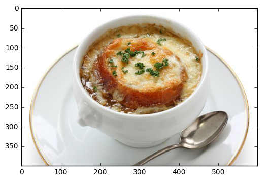
ローカルファイルからの予測
 pic_path = '/home/stratospark/Downloads/soup.jpg'
pic = img . imread ( pic_path )
preds = predict_10_crop ( np . array ( pic ), 0 )[ 0 ]
best_pred = collections . Counter ( preds ). most_common ( 1 )[ 0 ][ 0 ]
print ( ix_to_class [ best_pred ])
plt . imshow ( pic )
french_onion_soup
<matplotlib.image.AxesImage at 0x7fe2d59eb5c0>
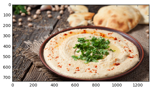
インターネット上の画像から予測します
 import urllib . request

@ interact
def predict_remote_image ( url = 'http://themodelhouse.tv/wp-content/uploads/2016/08/hummus.jpg' ):
    with urllib . request . urlopen ( url ) as f :
        pic = plt . imread ( f , format = 'jpg' )
        preds = predict_10_crop ( np . array ( pic ), 0 )[ 0 ]
        best_pred = collections . Counter ( preds ). most_common ( 1 )[ 0 ][ 0 ]
        print ( ix_to_class [ best_pred ])
        plt . imshow ( pic )
hummus
 with open ( 'model.json' , 'w' ) as f :
    f . write ( model . to_json ())
import json
json . dumps ( ix_to_class ) '{"0": "apple_pie", "1": "baby_back_ribs", "2": "baklava", "3": "beef_carpaccio", "4": "beef_tartare", "5": "beet_salad", "6": "beignets", "7": "bibimbap", "8": "bread_pudding", "9": "breakfast_burrito", "10": "bruschetta", "11": "caesar_salad", "12": "cannoli", "13": "caprese_salad", "14": "carrot_cake", "15": "ceviche", "16": "cheesecake", "17": "cheese_plate", "18": "chicken_curry", "19": "chicken_quesadilla", "20": "chicken_wings", "21": "chocolate_cake", "22": "chocolate_mousse", "23": "churros", "24": "clam_chowder", "25": "club_sandwich", "26": "crab_cakes", "27": "creme_brulee", "28": "croque_madame", "29": "cup_cakes", "30": "deviled_eggs", "31": "donuts", "32": "dumplings", "33": "edamame", "34": "eggs_benedict", "35": "escargots", "36": "falafel", "37": "filet_mignon", "38": "fish_and_chips", "39": "foie_gras", "40": "french_fries", "41": "french_onion_soup", "42": "french_toast", "43": "fried_calamari", "44": "fried_rice", "45": "frozen_yogurt", "46": "garlic_bread", "47": "gnocchi", "48": "greek_salad", "49": "grilled_cheese_sandwich", "50": "grilled_salmon", "51": "guacamole", "52": "gyoza", "53": "hamburger", "54": "hot_and_sour_soup", "55": "hot_dog", "56": "huevos_rancheros", "57": "hummus", "58": "ice_cream", "59": "lasagna", "60": "lobster_bisque", "61": "lobster_roll_sandwich", "62": "macaroni_and_cheese", "63": "macarons", "64": "miso_soup", "65": "mussels", "66": "nachos", "67": "omelette", "68": "onion_rings", "69": "oysters", "70": "pad_thai", "71": "paella", "72": "pancakes", "73": "panna_cotta", "74": "peking_duck", "75": "pho", "76": "pizza", "77": "pork_chop", "78": "poutine", "79": "prime_rib", "80": "pulled_pork_sandwich", "81": "ramen", "82": "ravioli", "83": "red_velvet_cake", "84": "risotto", "85": "samosa", "86": "sashimi", "87": "scallops", "88": "seaweed_salad", "89": "shrimp_and_grits", "90": "spaghetti_bolognese", "91": "spaghetti_carbonara", "92": "spring_rolls", "93": "steak", "94": "strawberry_shortcake", "95": "sushi", "96": "tacos", "97": "takoyaki", "98": "tiramisu", "99": "tuna_tartare", "100": "waffles"}'


