transformers interpret
v0.10.0
變形金剛解釋是一種模型解釋性工具,旨在專門與?變形金剛包。
與變壓器軟件包的理念一致,變壓器解釋允許僅以兩行解釋任何變壓器模型。解釋器可用於文本和計算機視覺模型。在筆記本電腦以及可保存的PNG和HTML文件中也可以使用可視化。
在此處查看簡化的演示應用程序
pip install transformers - interpret讓我們從初始化變壓器的模型和令牌器開始,然後通過“ sequenceCeclassificationExplainer”運行它。
在此示例中,我們使用了distilbert-base-uncased-finetuned-sst-2-english ,這是一種在情感分析任務上進行的Distilbert模型。
 from transformers import AutoModelForSequenceClassification , AutoTokenizer
model_name = "distilbert-base-uncased-finetuned-sst-2-english"
model = AutoModelForSequenceClassification . from_pretrained ( model_name )
tokenizer = AutoTokenizer . from_pretrained ( model_name )

# With both the model and tokenizer initialized we are now able to get explanations on an example text.

from transformers_interpret import SequenceClassificationExplainer
cls_explainer = SequenceClassificationExplainer (
    model ,
    tokenizer )
word_attributions = cls_explainer ( "I love you, I like you" )
哪個將返回以下單元列表:
 > >> word_attributions
[( '[CLS]' , 0.0 ),
 ( 'i' , 0.2778544699186709 ),
 ( 'love' , 0.7792370723380415 ),
 ( 'you' , 0.38560088858031094 ),
 ( ',' , - 0.01769750505546915 ),
 ( 'i' , 0.12071898121557832 ),
 ( 'like' , 0.19091105304734457 ),
 ( 'you' , 0.33994871536713467 ),
( '[SEP]' , 0.0 )]正歸因數字表明一個單詞對預測類有積極的貢獻,而負數表示一個單詞對預測類有負面影響。在這裡,我們可以看到我愛你最引起了人們的關注。
如果您想知道預測類實際是什麼,則可以使用predicted_class_index :
 > >> cls_explainer . predicted_class_index
array ( 1 )如果該模型具有每個類的標籤名稱,我們也可以使用predicted_class_name看到這些名稱:
 > >> cls_explainer . predicted_class_name
'POSITIVE' 有時,數字歸因可能很難閱讀,尤其是在有很多文本的情況下。為了幫助您,我們還提供了visualize()方法,該方法利用Captum在構建的VIZ庫中創建一個html文件,突出顯示屬性。
如果您在筆記本中,請訪問visualize()方法將在線顯示可視化。另外,您可以將filepath作為參數傳遞,並且將創建HTML文件,從而使您可以在瀏覽器中查看HTML的說明。
cls_explainer . visualize ( "distilbert_viz.html" )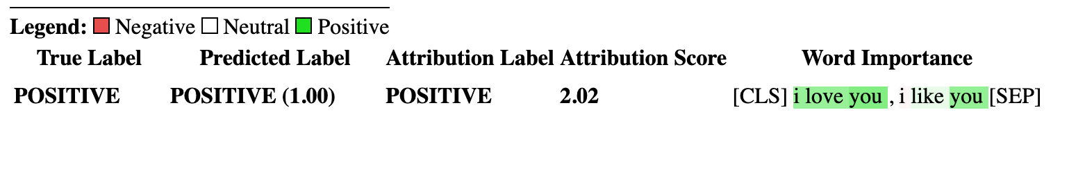
歸因解釋不僅限於預測類。讓我們測試一個更複雜的句子,其中包含混合情緒。
在下面的示例中,我們將class_name="NEGATIVE"傳遞給一個參數,表明我們希望為負類解釋屬性,而不管實際預測是什麼。有效地,因為這是我們獲得的二進制分類器。
 cls_explainer = SequenceClassificationExplainer ( model , tokenizer )
attributions = cls_explainer ( "I love you, I like you, I also kinda dislike you" , class_name = "NEGATIVE" )
在這種情況下, predicted_class_name仍然返回積極類的預測,因為該模型已經生成了相同的預測,但是儘管如此,我們還是有興趣查看負類別的屬性,無論預測結果如何。
 > >> cls_explainer . predicted_class_name
'POSITIVE'
但是,當我們可視化屬性時,我們可以看到“ ... Kinda不喜歡”一詞會導致對“負”類別的預測。
cls_explainer . visualize ( "distilbert_negative_attr.html" )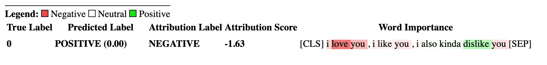
獲得不同類別的歸因對多類問題特別有見地,因為您可以檢查模型對模型的模型預測,並檢查模型“看”正確的事物。
有關此示例的詳細說明,請查看此多類分類筆記本。
PairwiseSequenceClassificationExplainer是SequenceClassificationExplainer Explainer的變體,該變體旨在與分類模型一起使用,這些分類模型期望輸入序列是兩個由模型的分離器令牌隔開的輸入。此的常見示例是NLI模型和交叉編碼器,它們通常用於對兩個輸入相似。
該解釋器使用構造函數中給出的模型和令牌來計算兩個傳遞的輸入text1和text2成對歸因。
同樣,由於成對序列分類的常見用例是比較兩個輸入相似性 - 此性質的模型通常只有一個單個輸出節點,而不是每個類的多個。成對序列分類具有一些有用的實用程序功能,以使解釋單節點輸出更清晰。
默認情況下,對於輸出單個節點的模型,屬性是相對於將分數推到1.0的輸入方面的屬性,但是,如果您想查看有關分數接近0.0的屬性,則可以通過flip_sign=True 。對於基於相似性的模型,這很有用,因為該模型可能會預測兩個輸入的分數接近0.0,在這種情況下,我們將翻轉屬性符號以解釋為什麼兩個輸入是不同的。
讓我們從句子轉換器提供的預先訓練的跨編碼器套件中初始化互編碼器模型和令牌。
在此示例中,我們使用的是"cross-encoder/ms-marco-MiniLM-L-6-v2" ,這是一種在MSMARCO數據集中訓練的高質量的跨編碼器,用於段落排名數據集,以解決問題答案和機器閱讀理解。
 from transformers import AutoModelForSequenceClassification , AutoTokenizer

from transformers_interpret import PairwiseSequenceClassificationExplainer

model = AutoModelForSequenceClassification . from_pretrained ( "cross-encoder/ms-marco-MiniLM-L-6-v2" )
tokenizer = AutoTokenizer . from_pretrained ( "cross-encoder/ms-marco-MiniLM-L-6-v2" )

pairwise_explainer = PairwiseSequenceClassificationExplainer ( model , tokenizer )

# the pairwise explainer requires two string inputs to be passed, in this case given the nature of the model
# we pass a query string and a context string. The question we are asking of our model is "does this context contain a valid answer to our question"
# the higher the score the better the fit.

query = "How many people live in Berlin?"
context = "Berlin has a population of 3,520,031 registered inhabitants in an area of 891.82 square kilometers."
pairwise_attr = pairwise_explainer ( query , context )
返回以下屬性:
 > >> pairwise_attr
[( '[CLS]' , 0.0 ),
 ( 'how' , - 0.037558652124213034 ),
 ( 'many' , - 0.40348581975409786 ),
 ( 'people' , - 0.29756140282349425 ),
 ( 'live' , - 0.48979015417391764 ),
 ( 'in' , - 0.17844527885888117 ),
 ( 'berlin' , 0.3737346097442739 ),
 ( '?' , - 0.2281428913480142 ),
 ( '[SEP]' , 0.0 ),
 ( 'berlin' , 0.18282430604641564 ),
 ( 'has' , 0.039114659489254834 ),
 ( 'a' , 0.0820056652212297 ),
 ( 'population' , 0.35712150914643026 ),
 ( 'of' , 0.09680870840224687 ),
 ( '3' , 0.04791760029513795 ),
 ( ',' , 0.040330986539774266 ),
 ( '520' , 0.16307677913176166 ),
 ( ',' , - 0.005919693904602767 ),
 ( '03' , 0.019431649515841844 ),
 ( '##1' , - 0.0243808667024702 ),
 ( 'registered' , 0.07748341753369632 ),
 ( 'inhabitants' , 0.23904087299731255 ),
 ( 'in' , 0.07553221327346359 ),
 ( 'an' , 0.033112821611999875 ),
 ( 'area' , - 0.025378852244447532 ),
 ( 'of' , 0.026526373859562906 ),
 ( '89' , 0.0030700151809002147 ),
 ( '##1' , - 0.000410387092186983 ),
 ( '.' , - 0.0193147139126114 ),
 ( '82' , 0.0073800833347678774 ),
 ( 'square' , 0.028988305990861576 ),
 ( 'kilometers' , 0.02071182933829008 ),
 ( '.' , - 0.025901070914318036 ),
( '[SEP]' , 0.0 )]可視化成對屬性與序列分類沒有什麼不同。我們可以看到,在query和context中, berlin一詞都有許多積極的歸因,以及在context中population和inhabitants一詞,我們的模型可以理解問題的文本上下文。
pairwise_explainer . visualize ( "cross_encoder_attr.html" )
如果我們更感興趣地突出顯示輸入屬性,這些輸入屬性將模型遠離該單個節點輸出的正類別類別,那麼我們可以通過:
pairwise_attr = explainer ( query , context , flip_sign = True )這簡單地將歸因的跡象倒出,以確保它們相對於輸出0而不是1的模型。
該解釋器是SequenceClassificationExplainer Explainer的擴展程序,因此與來自Transformers軟件包中的所有序列分類模型兼容。該解釋程序的關鍵更改是,它削減了模型配置中每個標籤的屬性,並將Word屬性WRT的字典返回到每個標籤中。 visualize()方法還顯示了一個屬性表,其屬性計算為每個標籤。
 from transformers import AutoModelForSequenceClassification , AutoTokenizer
from transformers_interpret import MultiLabelClassificationExplainer

model_name = "j-hartmann/emotion-english-distilroberta-base"
model = AutoModelForSequenceClassification . from_pretrained ( model_name )
tokenizer = AutoTokenizer . from_pretrained ( model_name )


cls_explainer = MultiLabelClassificationExplainer ( model , tokenizer )


word_attributions = cls_explainer ( "There were many aspects of the film I liked, but it was frightening and gross in parts. My parents hated it." )
這會產生一個單詞歸因的字典,將標籤映射到每個單詞的元組列表及其歸因分數。
 > >> word_attributions
{ 'anger' : [( '<s>' , 0.0 ),
           ( 'There' , 0.09002208622000409 ),
           ( 'were' , - 0.025129709879675187 ),
           ( 'many' , - 0.028852677974079328 ),
           ( 'aspects' , - 0.06341968013631565 ),
           ( 'of' , - 0.03587626320752477 ),
           ( 'the' , - 0.014813095892961287 ),
           ( 'film' , - 0.14087587475098232 ),
           ( 'I' , 0.007367876912617766 ),
           ( 'liked' , - 0.09816592066307557 ),
           ( ',' , - 0.014259517291745674 ),
           ( 'but' , - 0.08087144668471376 ),
           ( 'it' , - 0.10185214349220136 ),
           ( 'was' , - 0.07132244710777856 ),
           ( 'frightening' , - 0.4125361737439814 ),
           ( 'and' , - 0.021761663818889918 ),
           ( 'gross' , - 0.10423745223600908 ),
           ( 'in' , - 0.02383646952201854 ),
           ( 'parts' , - 0.027137622525091033 ),
           ( '.' , - 0.02960415694062459 ),
           ( 'My' , 0.05642774605113695 ),
           ( 'parents' , 0.11146648216326158 ),
           ( 'hated' , 0.8497975489280364 ),
           ( 'it' , 0.05358116678115284 ),
           ( '.' , - 0.013566277162080632 ),
           ( '' , 0.09293256725788422 ),
           ( '</s>' , 0.0 )],
 'disgust' : [( '<s>' , 0.0 ),
             ( 'There' , - 0.035296263203072 ),
             ( 'were' , - 0.010224922196739717 ),
             ( 'many' , - 0.03747571761725605 ),
             ( 'aspects' , 0.007696321643436715 ),
             ( 'of' , 0.0026740873113235107 ),
             ( 'the' , 0.0025752851265661335 ),
             ( 'film' , - 0.040890035285783645 ),
             ( 'I' , - 0.014710007408208579 ),
             ( 'liked' , 0.025696806663391577 ),
             ( ',' , - 0.00739107098314569 ),
             ( 'but' , 0.007353791868893654 ),
             ( 'it' , - 0.00821368234753605 ),
             ( 'was' , 0.005439709067819798 ),
             ( 'frightening' , - 0.8135974168445725 ),
             ( 'and' , - 0.002334953123414774 ),
             ( 'gross' , 0.2366024374426269 ),
             ( 'in' , 0.04314772995234148 ),
             ( 'parts' , 0.05590472194035334 ),
             ( '.' , - 0.04362554293972562 ),
             ( 'My' , - 0.04252694977895808 ),
             ( 'parents' , 0.051580790911406944 ),
             ( 'hated' , 0.5067406070057585 ),
             ( 'it' , 0.0527491071885104 ),
             ( '.' , - 0.008280280618652273 ),
             ( '' , 0.07412384603053103 ),
             ( '</s>' , 0.0 )],
 'fear' : [( '<s>' , 0.0 ),
          ( 'There' , - 0.019615758046045408 ),
          ( 'were' , 0.008033402634196246 ),
          ( 'many' , 0.027772367717635423 ),
          ( 'aspects' , 0.01334130725685673 ),
          ( 'of' , 0.009186049991879768 ),
          ( 'the' , 0.005828877177384549 ),
          ( 'film' , 0.09882910753644959 ),
          ( 'I' , 0.01753565003544039 ),
          ( 'liked' , 0.02062597344466885 ),
          ( ',' , - 0.004469530636560965 ),
          ( 'but' , - 0.019660439408176984 ),
          ( 'it' , 0.0488084071292538 ),
          ( 'was' , 0.03830859527501167 ),
          ( 'frightening' , 0.9526443954511705 ),
          ( 'and' , 0.02535156284103706 ),
          ( 'gross' , - 0.10635301961551227 ),
          ( 'in' , - 0.019190425328209065 ),
          ( 'parts' , - 0.01713006453323631 ),
          ( '.' , 0.015043169035757302 ),
          ( 'My' , 0.017068079071414916 ),
          ( 'parents' , - 0.0630781275517486 ),
          ( 'hated' , - 0.23630028921273583 ),
          ( 'it' , - 0.056057044429020306 ),
          ( '.' , 0.0015102052077844612 ),
          ( '' , - 0.010045048665404609 ),
          ( '</s>' , 0.0 )],
 'joy' : [( '<s>' , 0.0 ),
         ( 'There' , 0.04881772670614576 ),
         ( 'were' , - 0.0379316152427468 ),
         ( 'many' , - 0.007955371089444285 ),
         ( 'aspects' , 0.04437296429416574 ),
         ( 'of' , - 0.06407011137335743 ),
         ( 'the' , - 0.07331568926973099 ),
         ( 'film' , 0.21588462483311055 ),
         ( 'I' , 0.04885724513463952 ),
         ( 'liked' , 0.5309510543276107 ),
         ( ',' , 0.1339765195225006 ),
         ( 'but' , 0.09394079060730279 ),
         ( 'it' , - 0.1462792330432028 ),
         ( 'was' , - 0.1358591558323458 ),
         ( 'frightening' , - 0.22184169339341142 ),
         ( 'and' , - 0.07504142930419291 ),
         ( 'gross' , - 0.005472075984252812 ),
         ( 'in' , - 0.0942152657437379 ),
         ( 'parts' , - 0.19345218754215965 ),
         ( '.' , 0.11096247277185402 ),
         ( 'My' , 0.06604512262645984 ),
         ( 'parents' , 0.026376541098236207 ),
         ( 'hated' , - 0.4988319510231699 ),
         ( 'it' , - 0.17532499366236615 ),
         ( '.' , - 0.022609976138939034 ),
         ( '' , - 0.43417114685294833 ),
         ( '</s>' , 0.0 )],
 'neutral' : [( '<s>' , 0.0 ),
             ( 'There' , 0.045984598036642205 ),
             ( 'were' , 0.017142566357474697 ),
             ( 'many' , 0.011419348619472542 ),
             ( 'aspects' , 0.02558593440287365 ),
             ( 'of' , 0.0186162232003498 ),
             ( 'the' , 0.015616416841815963 ),
             ( 'film' , - 0.021190511300570092 ),
             ( 'I' , - 0.03572427925026324 ),
             ( 'liked' , 0.027062554960050455 ),
             ( ',' , 0.02089914209290366 ),
             ( 'but' , 0.025872618597570115 ),
             ( 'it' , - 0.002980407262316265 ),
             ( 'was' , - 0.022218157611174086 ),
             ( 'frightening' , - 0.2982516449116045 ),
             ( 'and' , - 0.01604643529040792 ),
             ( 'gross' , - 0.04573829263548096 ),
             ( 'in' , - 0.006511536166676108 ),
             ( 'parts' , - 0.011744224307968652 ),
             ( '.' , - 0.01817041167875332 ),
             ( 'My' , - 0.07362312722231429 ),
             ( 'parents' , - 0.06910711601816408 ),
             ( 'hated' , - 0.9418903509267312 ),
             ( 'it' , 0.022201795222373488 ),
             ( '.' , 0.025694319747309045 ),
             ( '' , 0.04276690822325994 ),
             ( '</s>' , 0.0 )],
 'sadness' : [( '<s>' , 0.0 ),
             ( 'There' , 0.028237893283377526 ),
             ( 'were' , - 0.04489910545229568 ),
             ( 'many' , 0.004996044977269471 ),
             ( 'aspects' , - 0.1231292680125582 ),
             ( 'of' , - 0.04552690725956671 ),
             ( 'the' , - 0.022077819961347042 ),
             ( 'film' , - 0.14155752357877663 ),
             ( 'I' , 0.04135347872193571 ),
             ( 'liked' , - 0.3097732540526099 ),
             ( ',' , 0.045114660009053134 ),
             ( 'but' , 0.0963352125332619 ),
             ( 'it' , - 0.08120617610094617 ),
             ( 'was' , - 0.08516150809170213 ),
             ( 'frightening' , - 0.10386889639962761 ),
             ( 'and' , - 0.03931986389970189 ),
             ( 'gross' , - 0.2145059013625132 ),
             ( 'in' , - 0.03465423285571697 ),
             ( 'parts' , - 0.08676627134611635 ),
             ( '.' , 0.19025217371906333 ),
             ( 'My' , 0.2582092561303794 ),
             ( 'parents' , 0.15432351476960307 ),
             ( 'hated' , 0.7262186310977987 ),
             ( 'it' , - 0.029160655114499095 ),
             ( '.' , - 0.002758524253450406 ),
             ( '' , - 0.33846410359182094 ),
             ( '</s>' , 0.0 )],
 'surprise' : [( '<s>' , 0.0 ),
              ( 'There' , 0.07196110795254315 ),
              ( 'were' , 0.1434314520711312 ),
              ( 'many' , 0.08812238369489701 ),
              ( 'aspects' , 0.013432396769890982 ),
              ( 'of' , - 0.07127508805657243 ),
              ( 'the' , - 0.14079766624810955 ),
              ( 'film' , - 0.16881201614906485 ),
              ( 'I' , 0.040595668935112135 ),
              ( 'liked' , 0.03239855530171577 ),
              ( ',' , - 0.17676382558158257 ),
              ( 'but' , - 0.03797939330341559 ),
              ( 'it' , - 0.029191325089641736 ),
              ( 'was' , 0.01758013584108571 ),
              ( 'frightening' , - 0.221738963726823 ),
              ( 'and' , - 0.05126920277135527 ),
              ( 'gross' , - 0.33986913466614044 ),
              ( 'in' , - 0.018180366628697 ),
              ( 'parts' , 0.02939418603252064 ),
              ( '.' , 0.018080129971003226 ),
              ( 'My' , - 0.08060162218059498 ),
              ( 'parents' , 0.04351719139081836 ),
              ( 'hated' , - 0.6919028585285265 ),
              ( 'it' , 0.0009574844165327357 ),
              ( '.' , - 0.059473118237873344 ),
              ( '' , - 0.465690452620123 ),
( '</s>' , 0.0 )]}有時,數字歸因可能很難閱讀,尤其是在有很多文本的情況下。為了幫助您,我們還提供了visualize()方法,該方法利用Captum在構建的VIZ庫中創建一個html文件,突出顯示屬性。對於此解釋程序,將顯示每個標籤的WRT。
如果您在筆記本中,請訪問visualize()方法將在線顯示可視化。另外,您可以將filepath作為參數傳遞,並且將創建HTML文件,從而使您可以在瀏覽器中查看HTML的說明。
cls_explainer . visualize ( "multilabel_viz.html" )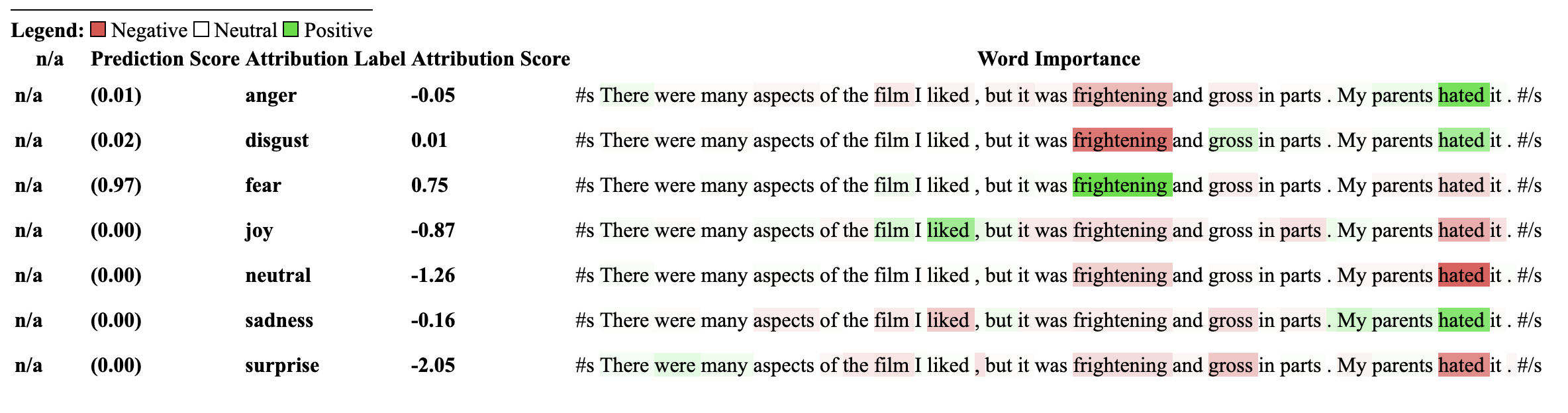
使用此解釋器的模型必須先前在NLI分類下游任務上進行培訓,並在模型配置中具有稱為“ Intailment”或“ Intailment”的標籤。
該解釋器允許計算零射擊分類(例如模型)的歸因。為了實現這一目標,我們使用擁抱面孔所採用的相同方法。對於那些不熟悉的方法,通過擁抱面孔來實現零射擊分類所使用的方式是通過利用NLI模型的“核心”標籤來實現的。這是一篇論文的鏈接,以說明更多有關它的信息。可以在模型中心上找到保證與此解釋器兼容的NLI模型列表。
讓我們從專門針對NLI任務進行了專門訓練的Transformers的序列分類模型和Tokenizer初始化,然後將其傳遞到ZeroshotClassification Explainer。
在此示例中,我們使用的是cross-encoder/nli-deberta-base ,它是在SNLI和NLI數據集數據集中訓練的Deberta基本模型的檢查點。該模型通常會預測句子對是一個需要,中性還是矛盾,但是對於零拍攝,我們只能查看零件標籤。
請注意,我們將自己的自定義標籤["finance", "technology", "sports"]傳遞給了類實例。可以傳遞任意數量的標籤,包括僅限一個標籤。可以通過predicted_label訪問最高的標籤分數,但是為每個標籤計算屬性本身。如果您想查看特定標籤的屬性,建議僅通過一個標籤傳遞該標籤,然後保證將確保計算標籤的wrt。
 from transformers import AutoModelForSequenceClassification , AutoTokenizer
from transformers_interpret import ZeroShotClassificationExplainer

tokenizer = AutoTokenizer . from_pretrained ( "cross-encoder/nli-deberta-base" )

model = AutoModelForSequenceClassification . from_pretrained ( "cross-encoder/nli-deberta-base" )


zero_shot_explainer = ZeroShotClassificationExplainer ( model , tokenizer )


word_attributions = zero_shot_explainer (
    "Today apple released the new Macbook showing off a range of new features found in the proprietary silicon chip computer. " ,
    labels = [ "finance" , "technology" , "sports" ],
)
這將返回每個標籤的歸因元組列表的以下命令:
 > >> word_attributions
{ 'finance' : [( '[CLS]' , 0.0 ),
  ( 'Today' , 0.144761198095125 ),
  ( 'apple' , 0.05008283286211926 ),
  ( 'released' , - 0.29790757134109724 ),
  ( 'the' , - 0.09931162582050683 ),
  ( 'new' , - 0.151252730475885 ),
  ( 'Mac' , 0.19431968978659608 ),
  ( 'book' , 0.059431761386793486 ),
  ( 'showing' , - 0.30754747734942633 ),
  ( 'off' , 0.0329034397830471 ),
  ( 'a' , 0.04198035048519715 ),
  ( 'range' , - 0.00413947940202566 ),
  ( 'of' , 0.7135069733740484 ),
  ( 'new' , 0.2294990755900286 ),
  ( 'features' , - 0.1523457769188503 ),
  ( 'found' , - 0.016804346228170633 ),
  ( 'in' , 0.1185751939327566 ),
  ( 'the' , - 0.06990875734316043 ),
  ( 'proprietary' , 0.16339657649559983 ),
  ( 'silicon' , 0.20461302470245252 ),
  ( 'chip' , 0.033304742383885574 ),
  ( 'computer' , - 0.058821677910955064 ),
  ( '.' , - 0.19741292299059068 )],
 'technology' : [( '[CLS]' , 0.0 ),
  ( 'Today' , 0.1261355373492264 ),
  ( 'apple' , - 0.06735584800073911 ),
  ( 'released' , - 0.37758515332894504 ),
  ( 'the' , - 0.16300368060788886 ),
  ( 'new' , - 0.1698884472100767 ),
  ( 'Mac' , 0.41505959302727347 ),
  ( 'book' , 0.321276307285395 ),
  ( 'showing' , - 0.2765988420377037 ),
  ( 'off' , 0.19388699112601515 ),
  ( 'a' , - 0.044676708673846766 ),
  ( 'range' , 0.05333370699507288 ),
  ( 'of' , 0.3654053610507722 ),
  ( 'new' , 0.3143976769670845 ),
  ( 'features' , 0.2108588137592185 ),
  ( 'found' , 0.004676960337191403 ),
  ( 'in' , 0.008026783104605233 ),
  ( 'the' , - 0.09961358108721637 ),
  ( 'proprietary' , 0.18816708356062326 ),
  ( 'silicon' , 0.13322691438800874 ),
  ( 'chip' , 0.015141805082331294 ),
  ( 'computer' , - 0.1321895049108681 ),
  ( '.' , - 0.17152401596638975 )],
 'sports' : [( '[CLS]' , 0.0 ),
  ( 'Today' , 0.11751821789941418 ),
  ( 'apple' , - 0.024552367058659215 ),
  ( 'released' , - 0.44706064525430567 ),
  ( 'the' , - 0.10163968191086448 ),
  ( 'new' , - 0.18590036257614642 ),
  ( 'Mac' , 0.0021649499897370725 ),
  ( 'book' , 0.009141161101058446 ),
  ( 'showing' , - 0.3073791152936541 ),
  ( 'off' , 0.0711051596941137 ),
  ( 'a' , 0.04153236257439005 ),
  ( 'range' , 0.01598478741712663 ),
  ( 'of' , 0.6632118834641558 ),
  ( 'new' , 0.2684728052423898 ),
  ( 'features' , - 0.10249856013919137 ),
  ( 'found' , - 0.032459999377294144 ),
  ( 'in' , 0.11078761617308391 ),
  ( 'the' , - 0.020530085754695244 ),
  ( 'proprietary' , 0.17968209761431955 ),
  ( 'silicon' , 0.19997909769476027 ),
  ( 'chip' , 0.04447720580439545 ),
  ( 'computer' , 0.018515748463790047 ),
  ( '.' , - 0.1686603393466192 )]}
我們可以發現哪個標籤已預測:
 > >> zero_shot_explainer . predicted_label
'technology' 對於ZeroShotClassificationExplainer Explainer,可視化()方法返回一個類似於SequenceClassificationExplainer的表,但每個標籤都具有屬性。
zero_shot_explainer . visualize ( "zero_shot.html" )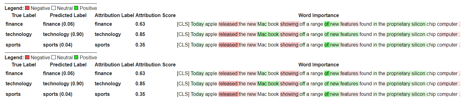
讓我們從初始化變形金剛的問題答案模型和令牌的開始,然後通過QuestionAnsweringExplainer運行它。
在此示例中,我們使用的是bert-large-uncased-whole-word-masking-finetuned-squad ,這是一個在小隊上進行的BERT模型。
 from transformers import AutoModelForQuestionAnswering , AutoTokenizer
from transformers_interpret import QuestionAnsweringExplainer

tokenizer = AutoTokenizer . from_pretrained ( "bert-large-uncased-whole-word-masking-finetuned-squad" )
model = AutoModelForQuestionAnswering . from_pretrained ( "bert-large-uncased-whole-word-masking-finetuned-squad" )

qa_explainer = QuestionAnsweringExplainer (
    model ,
    tokenizer ,
)

context = """
In Artificial Intelligence and machine learning, Natural Language Processing relates to the usage of machines to process and understand human language.
Many researchers currently work in this space.
"""

word_attributions = qa_explainer (
    "What is natural language processing ?" ,
    context ,
)
這將返回以下內容,其中包含詞語屬性,用於答案的預測啟動和結束位置。
 > >> word_attributions
{ 'start' : [( '[CLS]' , 0.0 ),
  ( 'what' , 0.9177170660377296 ),
  ( 'is' , 0.13382234898765258 ),
  ( 'natural' , 0.08061747350142005 ),
  ( 'language' , 0.013138062762511409 ),
  ( 'processing' , 0.11135923869816286 ),
  ( '?' , 0.00858057388924361 ),
  ( '[SEP]' , - 0.09646373141894966 ),
  ( 'in' , 0.01545633993975799 ),
  ( 'artificial' , 0.0472082598707737 ),
  ( 'intelligence' , 0.026687249355110867 ),
  ( 'and' , 0.01675371260058537 ),
  ( 'machine' , - 0.08429502436554961 ),
  ( 'learning' , 0.0044827685126163355 ),
  ( ',' , - 0.02401013152520878 ),
  ( 'natural' , - 0.0016756080249823537 ),
  ( 'language' , 0.0026815068421401885 ),
  ( 'processing' , 0.06773157580722854 ),
  ( 'relates' , 0.03884601576992908 ),
  ( 'to' , 0.009783797821526368 ),
  ( 'the' , - 0.026650922910540952 ),
  ( 'usage' , - 0.010675019721821147 ),
  ( 'of' , 0.015346787885898537 ),
  ( 'machines' , - 0.08278008270160107 ),
  ( 'to' , 0.12861387892768839 ),
  ( 'process' , 0.19540146386642743 ),
  ( 'and' , 0.009942879959615826 ),
  ( 'understand' , 0.006836894853320319 ),
  ( 'human' , 0.05020451122579102 ),
  ( 'language' , - 0.012980795199301 ),
  ( '.' , 0.00804358248127772 ),
  ( 'many' , 0.02259009321498161 ),
  ( 'researchers' , - 0.02351650942555469 ),
  ( 'currently' , 0.04484573078852946 ),
  ( 'work' , 0.00990399948294476 ),
  ( 'in' , 0.01806961211334615 ),
  ( 'this' , 0.13075899776164499 ),
  ( 'space' , 0.004298315347838973 ),
  ( '.' , - 0.003767904539347979 ),
  ( '[SEP]' , - 0.08891544093454595 )],
 'end' : [( '[CLS]' , 0.0 ),
  ( 'what' , 0.8227231947501547 ),
  ( 'is' , 0.0586864942952253 ),
  ( 'natural' , 0.0938903563379123 ),
  ( 'language' , 0.058596976016400674 ),
  ( 'processing' , 0.1632374290269829 ),
  ( '?' , 0.09695686057123237 ),
  ( '[SEP]' , - 0.11644447033554006 ),
  ( 'in' , - 0.03769172371919206 ),
  ( 'artificial' , 0.06736158404049886 ),
  ( 'intelligence' , 0.02496399001288386 ),
  ( 'and' , - 0.03526028847762427 ),
  ( 'machine' , - 0.20846431491771975 ),
  ( 'learning' , 0.00904892847529654 ),
  ( ',' , - 0.02949905488474854 ),
  ( 'natural' , 0.011024507784743872 ),
  ( 'language' , 0.0870741751282507 ),
  ( 'processing' , 0.11482449622317169 ),
  ( 'relates' , 0.05008962090922852 ),
  ( 'to' , 0.04079118393166258 ),
  ( 'the' , - 0.005069048880616451 ),
  ( 'usage' , - 0.011992752445836278 ),
  ( 'of' , 0.01715183316135495 ),
  ( 'machines' , - 0.29823535624026265 ),
  ( 'to' , - 0.0043760160855057925 ),
  ( 'process' , 0.10503217484645223 ),
  ( 'and' , 0.06840313586976698 ),
  ( 'understand' , 0.057184000619403944 ),
  ( 'human' , 0.0976805947708315 ),
  ( 'language' , 0.07031163646606695 ),
  ( '.' , 0.10494566513897102 ),
  ( 'many' , 0.019227154676079487 ),
  ( 'researchers' , - 0.038173913797800885 ),
  ( 'currently' , 0.03916641120002003 ),
  ( 'work' , 0.03705371672439422 ),
  ( 'in' , - 0.0003155975107591203 ),
  ( 'this' , 0.17254932354022232 ),
  ( 'space' , 0.0014311439625599323 ),
  ( '.' , 0.060637932829867736 ),
  ( '[SEP]' , - 0.09186286505530596 )]}
我們可以通過以下方式獲得預測答案的文本跨度:
 > >> qa_explainer . predicted_answer
'usage of machines to process and understand human language' 對於QuestionAnsweringExplainer ,可視化方法()方法返回帶有兩個行的表。第一行代表答案的開始位置的屬性,第二行代表答案的終端位置的屬性。
qa_explainer . visualize ( "bert_qa_viz.html" )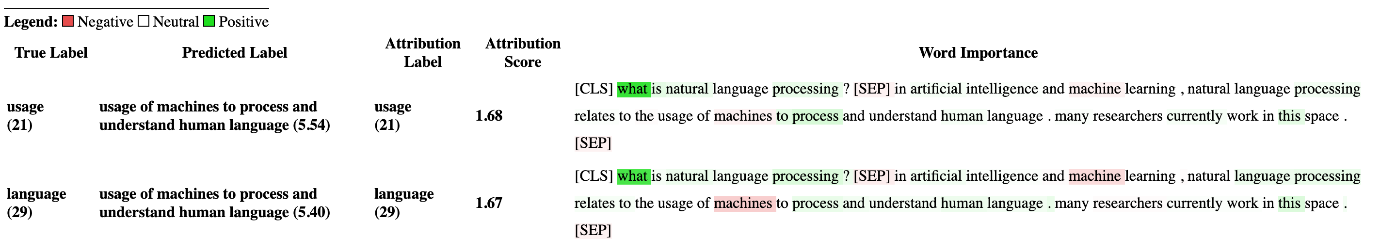
目前,這是一個正在積極開發的實驗解釋器,尚未進行全面測試。解釋器的API與歸因方法一樣,如果找到任何錯誤,請告訴我。
讓我們從初始化變形金剛的令牌類模型和令牌器,然後通過TokenClassificationExplainer運行它。
在此示例中,我們使用的是dslim/bert-base-NER ,這是在Conll-2003上名為“實體識別數據集”上進行的BERT模型。
 from transformers import AutoModelForTokenClassification , AutoTokenizer
from transformers_interpret import TokenClassificationExplainer

model = AutoModelForTokenClassification . from_pretrained ( 'dslim/bert-base-NER' )
tokenizer = AutoTokenizer . from_pretrained ( 'dslim/bert-base-NER' )

ner_explainer = TokenClassificationExplainer (
    model ,
    tokenizer ,
)

sample_text = "We visited Paris last weekend, where Emmanuel Macron lives."

word_attributions = ner_explainer ( sample_text , ignored_labels = [ 'O' ])為了減少計算的屬性數量,我們告訴解釋器忽略了標記的令牌,其預測標籤為'O' 。我們還可以告訴解釋器忽略某些索引,以提供列表作為參數ignored_indexes參數。
它將返回以下命令,其中包括預測標籤和每個令牌的歸因,除了被預測為“ O”的標籤:
 > >> word_attributions
{ 'paris' : { 'label' : 'B-LOC' ,
  'attribution_scores' : [( '[CLS]' , 0.0 ),
   ( 'we' , - 0.014352325471387907 ),
   ( 'visited' , 0.32915222186559123 ),
   ( 'paris' , 0.9086791784795596 ),
   ( 'last' , 0.15181203147624034 ),
   ( 'weekend' , 0.14400210630677038 ),
   ( ',' , 0.01899744327012935 ),
   ( 'where' , - 0.039402005463239465 ),
   ( 'emmanuel' , 0.061095284002642025 ),
   ( 'macro' , 0.004192922551105228 ),
   ( '##n' , 0.09446355513057757 ),
   ( 'lives' , - 0.028724312616455003 ),
   ( '.' , 0.08099007392937585 ),
   ( '[SEP]' , 0.0 )]},
 'emmanuel' : { 'label' : 'B-PER' ,
  'attribution_scores' : [( '[CLS]' , 0.0 ),
   ( 'we' , - 0.006933030636686712 ),
   ( 'visited' , 0.10396962390436904 ),
   ( 'paris' , 0.14540758744233165 ),
   ( 'last' , 0.08024018944451371 ),
   ( 'weekend' , 0.10687970996804418 ),
   ( ',' , 0.1793198466387937 ),
   ( 'where' , 0.3436407835483767 ),
   ( 'emmanuel' , 0.8774892642652167 ),
   ( 'macro' , 0.03559399361048316 ),
   ( '##n' , 0.1516315604785551 ),
   ( 'lives' , 0.07056441327498127 ),
   ( '.' , - 0.025820924624605487 ),
   ( '[SEP]' , 0.0 )]},
 'macro' : { 'label' : 'I-PER' ,
  'attribution_scores' : [( '[CLS]' , 0.0 ),
   ( 'we' , 0.05578067326280157 ),
   ( 'visited' , 0.00857021283406586 ),
   ( 'paris' , 0.16559056506114297 ),
   ( 'last' , 0.08285256685903823 ),
   ( 'weekend' , 0.10468727443796395 ),
   ( ',' , 0.09949509071515888 ),
   ( 'where' , 0.3642458274356929 ),
   ( 'emmanuel' , 0.7449335213978788 ),
   ( 'macro' , 0.3794625659183485 ),
   ( '##n' , - 0.2599031433800762 ),
   ( 'lives' , 0.20563450682196147 ),
   ( '.' , - 0.015607017319486929 ),
   ( '[SEP]' , 0.0 )]},
 '##n' : { 'label' : 'I-PER' ,
  'attribution_scores' : [( '[CLS]' , 0.0 ),
   ( 'we' , 0.025194121717285252 ),
   ( 'visited' , - 0.007415022865239864 ),
   ( 'paris' , 0.09478357303107598 ),
   ( 'last' , 0.06927939834474463 ),
   ( 'weekend' , 0.0672008033510708 ),
   ( ',' , 0.08316907214363504 ),
   ( 'where' , 0.3784915854680165 ),
   ( 'emmanuel' , 0.7729352621546081 ),
   ( 'macro' , 0.4148652759139777 ),
   ( '##n' , - 0.20853534512145033 ),
   ( 'lives' , 0.09445057087678274 ),
   ( '.' , - 0.094274985907366 ),
   ( '[SEP]' , 0.0 )]},
 '[SEP]' : { 'label' : 'B-LOC' ,
  'attribution_scores' : [( '[CLS]' , 0.0 ),
   ( 'we' , - 0.3694351403796742 ),
   ( 'visited' , 0.1699038407402483 ),
   ( 'paris' , 0.5461587414992369 ),
   ( 'last' , 0.0037948102770307517 ),
   ( 'weekend' , 0.1628100955702496 ),
   ( ',' , 0.4513093410909263 ),
   ( 'where' , - 0.09577409464161038 ),
   ( 'emmanuel' , 0.48499459835388914 ),
   ( 'macro' , - 0.13528905587653023 ),
   ( '##n' , 0.14362969934754344 ),
   ( 'lives' , - 0.05758007024257254 ),
   ( '.' , - 0.13970977266152554 ),
( '[SEP]' , 0.0 )]}}對於TokenClassificationExplainer開發器,可視化方法()方法返回具有與令牌一樣多的行的表。
ner_explainer . visualize ( "bert_ner_viz.html" )
有關TokenClassificationExplainer工作方式的更多詳細信息,您可以查看筆記本電腦/ner_example.ipynb。
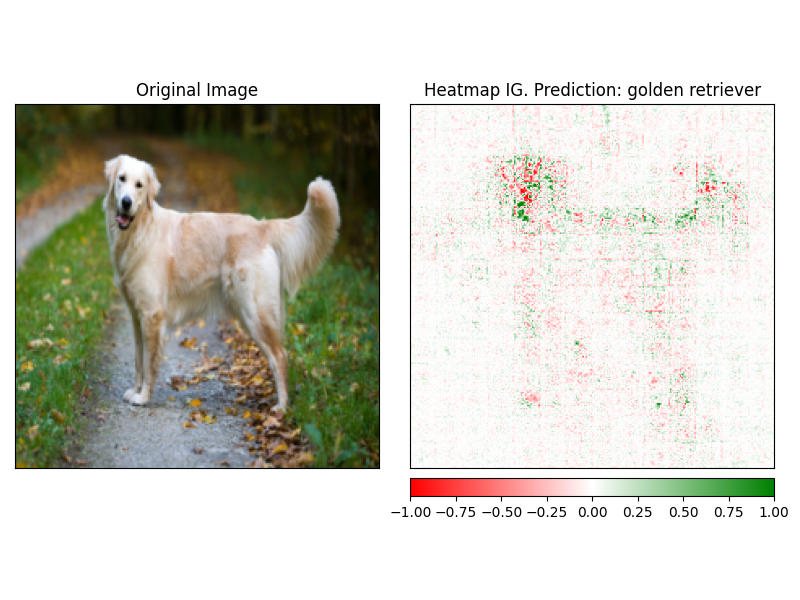
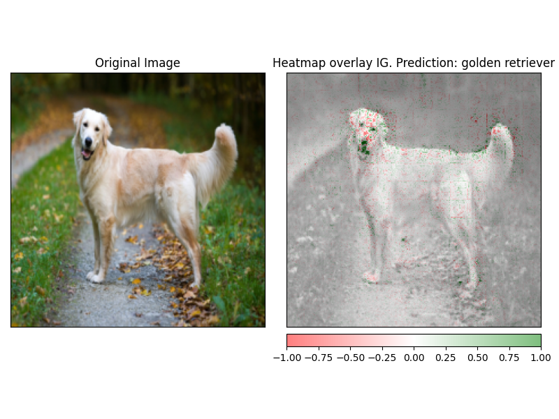
ImageClassificationExplainer旨在與經過訓練用於圖像分類(SWIN,VIT等)的所有模型一起使用。它為該圖像中的每個像素提供了歸因,可以使用visualize方法中內置的解釋器輕鬆可視化。
初始化圖像分類非常簡單,您所需要的只是圖像分類模型固定或培訓,可與HuggingFace及其特徵提取器一起使用。
在此示例中,我們使用的是google/vit-base-patch16-224 ,這是在Imagenet-21K上預先訓練的視覺變壓器(VIT)模型,可預測1000個可能的類別。
 from transformers import AutoFeatureExtractor , AutoModelForImageClassification
from transformers_interpret import ImageClassificationExplainer
from PIL import Image
import requests

model_name = "google/vit-base-patch16-224"
model = AutoModelForImageClassification . from_pretrained ( model_name )
feature_extractor = AutoFeatureExtractor . from_pretrained ( model_name )

# With both the model and feature extractor initialized we are now able to get explanations on an image, we will use a simple image of a golden retriever.
image_link = "https://imagesvc.meredithcorp.io/v3/mm/image?url=https%3A%2F%2Fstatic.onecms.io%2Fwp-content%2Fuploads%2Fsites%2F47%2F2020%2F08%2F16%2Fgolden-retriever-177213599-2000.jpg"

image = Image . open ( requests . get ( image_link , stream = True ). raw )

image_classification_explainer = ImageClassificationExplainer ( model = model , feature_extractor = feature_extractor )

image_attributions = image_classification_explainer (
    image
)

print ( image_attributions . shape )
哪個將返回以下單元列表:
> >> torch . Size ([ 1 , 3 , 224 , 224 ])因為我們正在處理圖像的可視化比文本模型更簡單。
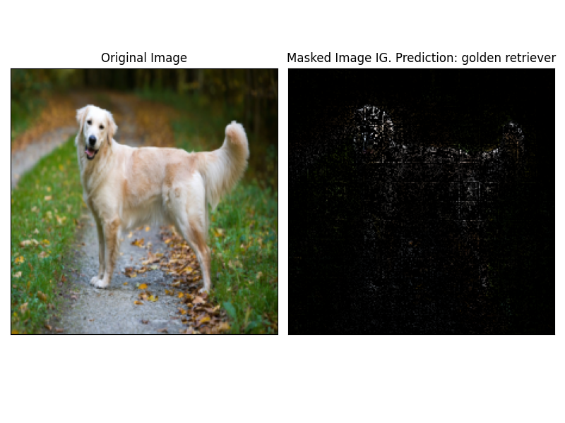
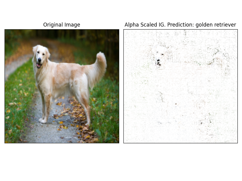
使用解釋器的visualize方法可以輕鬆地可視化attrbution。當前有4種支持的可視化方法。
heatmap - 使用圖像的尺寸繪製正歸因和負歸因的熱圖。overlay - 熱圖被覆蓋在原始圖像的灰度版本上masked_image屬性的絕對值用於通過原始圖像創建掩碼alpha_scaling將每個像素的Alpha通道(透明度)設置為等於歸一化的歸因值。 image_classification_explainer . visualize (
method = "heatmap" ,
side_by_side = True ,
outlier_threshold = 0.03
)
 image_classification_explainer . visualize (
    method = "overlay" ,
    side_by_side = True ,
    outlier_threshold = 0.03

)
 image_classification_explainer . visualize (
    method = "masked_image" ,
    side_by_side = True ,
    outlier_threshold = 0.03

)
 image_classification_explainer . visualize (
    method = "alpha_scaling" ,
    side_by_side = True ,
    outlier_threshold = 0.03

)
該軟件包仍在積極開發中,並且有更多計劃。對於1.0.0版本,我們的目標是:
如果您想做出貢獻,請查看我們的貢獻指南
該存儲庫的維護者是@cdpierse。
如果您有任何疑問,建議或想做出貢獻(請這樣做?),請隨時通過[email protected]與您取得聯繫。
如果您發現模型的解釋性和解釋性有趣,我也強烈建議您檢查Captum。
該包裹坐落在Pytorch Captum和擁抱臉的團隊所做的令人難以置信的工作的肩膀上,如果不是因為他們在ML和模型可解釋性領域所做的出色工作,就不存在。
該軟件包中的所有屬性都是使用Pytorch的解釋性軟件包CAPTUM計算的。有關與Captum相關的一些有用鏈接,請參見下文。
集成梯度(IG)和IT層積分梯度(LIG)的變體是當前構建變壓器解釋的核心歸因方法。以下是一些有用的資源,包括原始論文和一些視頻鏈接,解釋了內部力學。如果您對變形金剛內部發生的事情感到好奇,我強烈建議您查看至少其中一種資源。
Captum鏈接
以下是我用來幫助我使用Captum將此包裝在一起的一些鏈接。感謝@davidefiocco的洞察力。


