transformers interpret
v0.10.0
变形金刚解释是一种模型解释性工具,旨在专门与?变形金刚包。
与变压器软件包的理念一致,变压器解释允许仅以两行解释任何变压器模型。解释器可用于文本和计算机视觉模型。在笔记本电脑以及可保存的PNG和HTML文件中也可以使用可视化。
在此处查看简化的演示应用程序
pip install transformers - interpret让我们从初始化变压器的模型和令牌器开始,然后通过“ sequenceCeclassificationExplainer”运行它。
在此示例中,我们使用了distilbert-base-uncased-finetuned-sst-2-english ,这是一种在情感分析任务上进行的Distilbert模型。
 from transformers import AutoModelForSequenceClassification , AutoTokenizer
model_name = "distilbert-base-uncased-finetuned-sst-2-english"
model = AutoModelForSequenceClassification . from_pretrained ( model_name )
tokenizer = AutoTokenizer . from_pretrained ( model_name )

# With both the model and tokenizer initialized we are now able to get explanations on an example text.

from transformers_interpret import SequenceClassificationExplainer
cls_explainer = SequenceClassificationExplainer (
    model ,
    tokenizer )
word_attributions = cls_explainer ( "I love you, I like you" )
哪个将返回以下单元列表:
 > >> word_attributions
[( '[CLS]' , 0.0 ),
 ( 'i' , 0.2778544699186709 ),
 ( 'love' , 0.7792370723380415 ),
 ( 'you' , 0.38560088858031094 ),
 ( ',' , - 0.01769750505546915 ),
 ( 'i' , 0.12071898121557832 ),
 ( 'like' , 0.19091105304734457 ),
 ( 'you' , 0.33994871536713467 ),
( '[SEP]' , 0.0 )]正归因数字表明一个单词对预测类有积极的贡献,而负数表示一个单词对预测类有负面影响。在这里,我们可以看到我爱你最引起了人们的关注。
如果您想知道预测类实际是什么,则可以使用predicted_class_index :
 > >> cls_explainer . predicted_class_index
array ( 1 )如果该模型具有每个类的标签名称,我们也可以使用predicted_class_name看到这些名称:
 > >> cls_explainer . predicted_class_name
'POSITIVE' 有时,数字归因可能很难阅读,尤其是在有很多文本的情况下。为了帮助您,我们还提供了visualize()方法,该方法利用Captum在构建的VIZ库中创建一个html文件,突出显示属性。
如果您在笔记本中,请访问visualize()方法将在线显示可视化。另外,您可以将filepath作为参数传递,并且将创建HTML文件,从而使您可以在浏览器中查看HTML的说明。
cls_explainer . visualize ( "distilbert_viz.html" )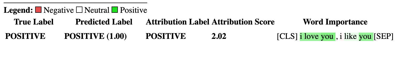
归因解释不仅限于预测类。让我们测试一个更复杂的句子,其中包含混合情绪。
在下面的示例中,我们将class_name="NEGATIVE"传递给一个参数,表明我们希望为负类解释属性,而不管实际预测是什么。有效地,因为这是我们获得的二进制分类器。
 cls_explainer = SequenceClassificationExplainer ( model , tokenizer )
attributions = cls_explainer ( "I love you, I like you, I also kinda dislike you" , class_name = "NEGATIVE" )
在这种情况下, predicted_class_name仍然返回积极类的预测,因为该模型已经生成了相同的预测,但是尽管如此,我们还是有兴趣查看负类别的属性,无论预测结果如何。
 > >> cls_explainer . predicted_class_name
'POSITIVE'
但是,当我们可视化属性时,我们可以看到“ ... Kinda不喜欢”一词会导致对“负”类别的预测。
cls_explainer . visualize ( "distilbert_negative_attr.html" )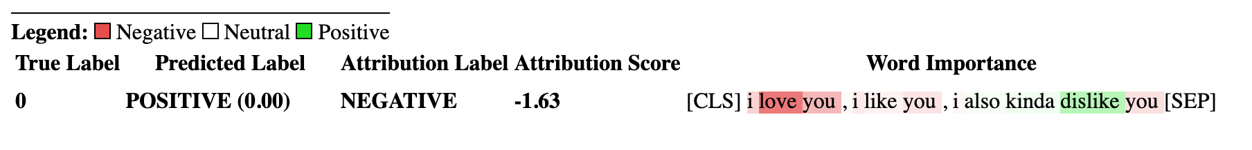
获得不同类别的归因对多类问题特别有见地,因为您可以检查模型对模型的模型预测,并检查模型“看”正确的事物。
有关此示例的详细说明,请查看此多类分类笔记本。
PairwiseSequenceClassificationExplainer是SequenceClassificationExplainer Explainer的变体,该变体旨在与分类模型一起使用,这些分类模型期望输入序列是两个由模型的分离器令牌隔开的输入。此的常见示例是NLI模型和交叉编码器,它们通常用于对两个输入相似。
该解释器使用构造函数中给出的模型和令牌来计算两个传递的输入text1和text2成对归因。
同样,由于成对序列分类的常见用例是比较两个输入相似性 - 此性质的模型通常只有一个单个输出节点,而不是每个类的多个。成对序列分类具有一些有用的实用程序功能,以使解释单节点输出更清晰。
默认情况下,对于输出单个节点的模型,属性是相对于将分数推到1.0的输入方面的属性,但是,如果您想查看有关分数接近0.0的属性,则可以通过flip_sign=True 。对于基于相似性的模型,这很有用,因为该模型可能会预测两个输入的分数接近0.0,在这种情况下,我们将翻转属性符号以解释为什么两个输入是不同的。
让我们从句子转换器提供的预先训练的跨编码器套件中初始化互编码器模型和令牌。
在此示例中,我们使用的是"cross-encoder/ms-marco-MiniLM-L-6-v2" ,这是一种在MSMARCO数据集中训练的高质量的跨编码器,用于段落排名数据集,以解决问题答案和机器阅读理解。
 from transformers import AutoModelForSequenceClassification , AutoTokenizer

from transformers_interpret import PairwiseSequenceClassificationExplainer

model = AutoModelForSequenceClassification . from_pretrained ( "cross-encoder/ms-marco-MiniLM-L-6-v2" )
tokenizer = AutoTokenizer . from_pretrained ( "cross-encoder/ms-marco-MiniLM-L-6-v2" )

pairwise_explainer = PairwiseSequenceClassificationExplainer ( model , tokenizer )

# the pairwise explainer requires two string inputs to be passed, in this case given the nature of the model
# we pass a query string and a context string. The question we are asking of our model is "does this context contain a valid answer to our question"
# the higher the score the better the fit.

query = "How many people live in Berlin?"
context = "Berlin has a population of 3,520,031 registered inhabitants in an area of 891.82 square kilometers."
pairwise_attr = pairwise_explainer ( query , context )
返回以下属性:
 > >> pairwise_attr
[( '[CLS]' , 0.0 ),
 ( 'how' , - 0.037558652124213034 ),
 ( 'many' , - 0.40348581975409786 ),
 ( 'people' , - 0.29756140282349425 ),
 ( 'live' , - 0.48979015417391764 ),
 ( 'in' , - 0.17844527885888117 ),
 ( 'berlin' , 0.3737346097442739 ),
 ( '?' , - 0.2281428913480142 ),
 ( '[SEP]' , 0.0 ),
 ( 'berlin' , 0.18282430604641564 ),
 ( 'has' , 0.039114659489254834 ),
 ( 'a' , 0.0820056652212297 ),
 ( 'population' , 0.35712150914643026 ),
 ( 'of' , 0.09680870840224687 ),
 ( '3' , 0.04791760029513795 ),
 ( ',' , 0.040330986539774266 ),
 ( '520' , 0.16307677913176166 ),
 ( ',' , - 0.005919693904602767 ),
 ( '03' , 0.019431649515841844 ),
 ( '##1' , - 0.0243808667024702 ),
 ( 'registered' , 0.07748341753369632 ),
 ( 'inhabitants' , 0.23904087299731255 ),
 ( 'in' , 0.07553221327346359 ),
 ( 'an' , 0.033112821611999875 ),
 ( 'area' , - 0.025378852244447532 ),
 ( 'of' , 0.026526373859562906 ),
 ( '89' , 0.0030700151809002147 ),
 ( '##1' , - 0.000410387092186983 ),
 ( '.' , - 0.0193147139126114 ),
 ( '82' , 0.0073800833347678774 ),
 ( 'square' , 0.028988305990861576 ),
 ( 'kilometers' , 0.02071182933829008 ),
 ( '.' , - 0.025901070914318036 ),
( '[SEP]' , 0.0 )]可视化成对属性与序列分类没有什么不同。我们可以看到,在query和context中, berlin一词都有许多积极的归因,以及在context中population和inhabitants一词,我们的模型可以理解问题的文本上下文。
pairwise_explainer . visualize ( "cross_encoder_attr.html" )
如果我们更感兴趣地突出显示输入属性,这些输入属性将模型远离该单个节点输出的正类别类别,那么我们可以通过:
pairwise_attr = explainer ( query , context , flip_sign = True )这简单地将归因的迹象倒出,以确保它们相对于输出0而不是1的模型。
该解释器是SequenceClassificationExplainer Explainer的扩展程序,因此与来自Transformers软件包中的所有序列分类模型兼容。该解释程序的关键更改是,它削减了模型配置中每个标签的属性,并将Word属性WRT的字典返回到每个标签中。 visualize()方法还显示了一个属性表,其属性计算为每个标签。
 from transformers import AutoModelForSequenceClassification , AutoTokenizer
from transformers_interpret import MultiLabelClassificationExplainer

model_name = "j-hartmann/emotion-english-distilroberta-base"
model = AutoModelForSequenceClassification . from_pretrained ( model_name )
tokenizer = AutoTokenizer . from_pretrained ( model_name )


cls_explainer = MultiLabelClassificationExplainer ( model , tokenizer )


word_attributions = cls_explainer ( "There were many aspects of the film I liked, but it was frightening and gross in parts. My parents hated it." )
这会产生一个单词归因的字典,将标签映射到每个单词的元组列表及其归因分数。
 > >> word_attributions
{ 'anger' : [( '<s>' , 0.0 ),
           ( 'There' , 0.09002208622000409 ),
           ( 'were' , - 0.025129709879675187 ),
           ( 'many' , - 0.028852677974079328 ),
           ( 'aspects' , - 0.06341968013631565 ),
           ( 'of' , - 0.03587626320752477 ),
           ( 'the' , - 0.014813095892961287 ),
           ( 'film' , - 0.14087587475098232 ),
           ( 'I' , 0.007367876912617766 ),
           ( 'liked' , - 0.09816592066307557 ),
           ( ',' , - 0.014259517291745674 ),
           ( 'but' , - 0.08087144668471376 ),
           ( 'it' , - 0.10185214349220136 ),
           ( 'was' , - 0.07132244710777856 ),
           ( 'frightening' , - 0.4125361737439814 ),
           ( 'and' , - 0.021761663818889918 ),
           ( 'gross' , - 0.10423745223600908 ),
           ( 'in' , - 0.02383646952201854 ),
           ( 'parts' , - 0.027137622525091033 ),
           ( '.' , - 0.02960415694062459 ),
           ( 'My' , 0.05642774605113695 ),
           ( 'parents' , 0.11146648216326158 ),
           ( 'hated' , 0.8497975489280364 ),
           ( 'it' , 0.05358116678115284 ),
           ( '.' , - 0.013566277162080632 ),
           ( '' , 0.09293256725788422 ),
           ( '</s>' , 0.0 )],
 'disgust' : [( '<s>' , 0.0 ),
             ( 'There' , - 0.035296263203072 ),
             ( 'were' , - 0.010224922196739717 ),
             ( 'many' , - 0.03747571761725605 ),
             ( 'aspects' , 0.007696321643436715 ),
             ( 'of' , 0.0026740873113235107 ),
             ( 'the' , 0.0025752851265661335 ),
             ( 'film' , - 0.040890035285783645 ),
             ( 'I' , - 0.014710007408208579 ),
             ( 'liked' , 0.025696806663391577 ),
             ( ',' , - 0.00739107098314569 ),
             ( 'but' , 0.007353791868893654 ),
             ( 'it' , - 0.00821368234753605 ),
             ( 'was' , 0.005439709067819798 ),
             ( 'frightening' , - 0.8135974168445725 ),
             ( 'and' , - 0.002334953123414774 ),
             ( 'gross' , 0.2366024374426269 ),
             ( 'in' , 0.04314772995234148 ),
             ( 'parts' , 0.05590472194035334 ),
             ( '.' , - 0.04362554293972562 ),
             ( 'My' , - 0.04252694977895808 ),
             ( 'parents' , 0.051580790911406944 ),
             ( 'hated' , 0.5067406070057585 ),
             ( 'it' , 0.0527491071885104 ),
             ( '.' , - 0.008280280618652273 ),
             ( '' , 0.07412384603053103 ),
             ( '</s>' , 0.0 )],
 'fear' : [( '<s>' , 0.0 ),
          ( 'There' , - 0.019615758046045408 ),
          ( 'were' , 0.008033402634196246 ),
          ( 'many' , 0.027772367717635423 ),
          ( 'aspects' , 0.01334130725685673 ),
          ( 'of' , 0.009186049991879768 ),
          ( 'the' , 0.005828877177384549 ),
          ( 'film' , 0.09882910753644959 ),
          ( 'I' , 0.01753565003544039 ),
          ( 'liked' , 0.02062597344466885 ),
          ( ',' , - 0.004469530636560965 ),
          ( 'but' , - 0.019660439408176984 ),
          ( 'it' , 0.0488084071292538 ),
          ( 'was' , 0.03830859527501167 ),
          ( 'frightening' , 0.9526443954511705 ),
          ( 'and' , 0.02535156284103706 ),
          ( 'gross' , - 0.10635301961551227 ),
          ( 'in' , - 0.019190425328209065 ),
          ( 'parts' , - 0.01713006453323631 ),
          ( '.' , 0.015043169035757302 ),
          ( 'My' , 0.017068079071414916 ),
          ( 'parents' , - 0.0630781275517486 ),
          ( 'hated' , - 0.23630028921273583 ),
          ( 'it' , - 0.056057044429020306 ),
          ( '.' , 0.0015102052077844612 ),
          ( '' , - 0.010045048665404609 ),
          ( '</s>' , 0.0 )],
 'joy' : [( '<s>' , 0.0 ),
         ( 'There' , 0.04881772670614576 ),
         ( 'were' , - 0.0379316152427468 ),
         ( 'many' , - 0.007955371089444285 ),
         ( 'aspects' , 0.04437296429416574 ),
         ( 'of' , - 0.06407011137335743 ),
         ( 'the' , - 0.07331568926973099 ),
         ( 'film' , 0.21588462483311055 ),
         ( 'I' , 0.04885724513463952 ),
         ( 'liked' , 0.5309510543276107 ),
         ( ',' , 0.1339765195225006 ),
         ( 'but' , 0.09394079060730279 ),
         ( 'it' , - 0.1462792330432028 ),
         ( 'was' , - 0.1358591558323458 ),
         ( 'frightening' , - 0.22184169339341142 ),
         ( 'and' , - 0.07504142930419291 ),
         ( 'gross' , - 0.005472075984252812 ),
         ( 'in' , - 0.0942152657437379 ),
         ( 'parts' , - 0.19345218754215965 ),
         ( '.' , 0.11096247277185402 ),
         ( 'My' , 0.06604512262645984 ),
         ( 'parents' , 0.026376541098236207 ),
         ( 'hated' , - 0.4988319510231699 ),
         ( 'it' , - 0.17532499366236615 ),
         ( '.' , - 0.022609976138939034 ),
         ( '' , - 0.43417114685294833 ),
         ( '</s>' , 0.0 )],
 'neutral' : [( '<s>' , 0.0 ),
             ( 'There' , 0.045984598036642205 ),
             ( 'were' , 0.017142566357474697 ),
             ( 'many' , 0.011419348619472542 ),
             ( 'aspects' , 0.02558593440287365 ),
             ( 'of' , 0.0186162232003498 ),
             ( 'the' , 0.015616416841815963 ),
             ( 'film' , - 0.021190511300570092 ),
             ( 'I' , - 0.03572427925026324 ),
             ( 'liked' , 0.027062554960050455 ),
             ( ',' , 0.02089914209290366 ),
             ( 'but' , 0.025872618597570115 ),
             ( 'it' , - 0.002980407262316265 ),
             ( 'was' , - 0.022218157611174086 ),
             ( 'frightening' , - 0.2982516449116045 ),
             ( 'and' , - 0.01604643529040792 ),
             ( 'gross' , - 0.04573829263548096 ),
             ( 'in' , - 0.006511536166676108 ),
             ( 'parts' , - 0.011744224307968652 ),
             ( '.' , - 0.01817041167875332 ),
             ( 'My' , - 0.07362312722231429 ),
             ( 'parents' , - 0.06910711601816408 ),
             ( 'hated' , - 0.9418903509267312 ),
             ( 'it' , 0.022201795222373488 ),
             ( '.' , 0.025694319747309045 ),
             ( '' , 0.04276690822325994 ),
             ( '</s>' , 0.0 )],
 'sadness' : [( '<s>' , 0.0 ),
             ( 'There' , 0.028237893283377526 ),
             ( 'were' , - 0.04489910545229568 ),
             ( 'many' , 0.004996044977269471 ),
             ( 'aspects' , - 0.1231292680125582 ),
             ( 'of' , - 0.04552690725956671 ),
             ( 'the' , - 0.022077819961347042 ),
             ( 'film' , - 0.14155752357877663 ),
             ( 'I' , 0.04135347872193571 ),
             ( 'liked' , - 0.3097732540526099 ),
             ( ',' , 0.045114660009053134 ),
             ( 'but' , 0.0963352125332619 ),
             ( 'it' , - 0.08120617610094617 ),
             ( 'was' , - 0.08516150809170213 ),
             ( 'frightening' , - 0.10386889639962761 ),
             ( 'and' , - 0.03931986389970189 ),
             ( 'gross' , - 0.2145059013625132 ),
             ( 'in' , - 0.03465423285571697 ),
             ( 'parts' , - 0.08676627134611635 ),
             ( '.' , 0.19025217371906333 ),
             ( 'My' , 0.2582092561303794 ),
             ( 'parents' , 0.15432351476960307 ),
             ( 'hated' , 0.7262186310977987 ),
             ( 'it' , - 0.029160655114499095 ),
             ( '.' , - 0.002758524253450406 ),
             ( '' , - 0.33846410359182094 ),
             ( '</s>' , 0.0 )],
 'surprise' : [( '<s>' , 0.0 ),
              ( 'There' , 0.07196110795254315 ),
              ( 'were' , 0.1434314520711312 ),
              ( 'many' , 0.08812238369489701 ),
              ( 'aspects' , 0.013432396769890982 ),
              ( 'of' , - 0.07127508805657243 ),
              ( 'the' , - 0.14079766624810955 ),
              ( 'film' , - 0.16881201614906485 ),
              ( 'I' , 0.040595668935112135 ),
              ( 'liked' , 0.03239855530171577 ),
              ( ',' , - 0.17676382558158257 ),
              ( 'but' , - 0.03797939330341559 ),
              ( 'it' , - 0.029191325089641736 ),
              ( 'was' , 0.01758013584108571 ),
              ( 'frightening' , - 0.221738963726823 ),
              ( 'and' , - 0.05126920277135527 ),
              ( 'gross' , - 0.33986913466614044 ),
              ( 'in' , - 0.018180366628697 ),
              ( 'parts' , 0.02939418603252064 ),
              ( '.' , 0.018080129971003226 ),
              ( 'My' , - 0.08060162218059498 ),
              ( 'parents' , 0.04351719139081836 ),
              ( 'hated' , - 0.6919028585285265 ),
              ( 'it' , 0.0009574844165327357 ),
              ( '.' , - 0.059473118237873344 ),
              ( '' , - 0.465690452620123 ),
( '</s>' , 0.0 )]}有时,数字归因可能很难阅读,尤其是在有很多文本的情况下。为了帮助您,我们还提供了visualize()方法,该方法利用Captum在构建的VIZ库中创建一个html文件,突出显示属性。对于此解释程序,将显示每个标签的WRT。
如果您在笔记本中,请访问visualize()方法将在线显示可视化。另外,您可以将filepath作为参数传递,并且将创建HTML文件,从而使您可以在浏览器中查看HTML的说明。
cls_explainer . visualize ( "multilabel_viz.html" )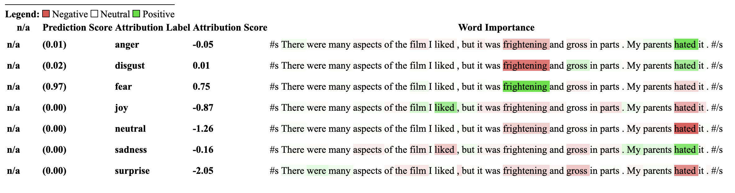
使用此解释器的模型必须先前在NLI分类下游任务上进行培训,并在模型配置中具有称为“ Intailment”或“ Intailment”的标签。
该解释器允许计算零射击分类(例如模型)的归因。为了实现这一目标,我们使用拥抱面孔所采用的相同方法。对于那些不熟悉的方法,通过拥抱面孔来实现零射击分类所使用的方式是通过利用NLI模型的“核心”标签来实现的。这是一篇论文的链接,以说明更多有关它的信息。可以在模型中心上找到保证与此解释器兼容的NLI模型列表。
让我们从专门针对NLI任务进行了专门训练的Transformers的序列分类模型和Tokenizer初始化,然后将其传递到ZeroshotClassification Explainer。
在此示例中,我们使用的是cross-encoder/nli-deberta-base ,它是在SNLI和NLI数据集数据集中训练的Deberta基本模型的检查点。该模型通常会预测句子对是一个需要,中性还是矛盾,但是对于零拍摄,我们只能查看零件标签。
请注意,我们将自己的自定义标签["finance", "technology", "sports"]传递给了类实例。可以传递任意数量的标签,包括仅限一个标签。可以通过predicted_label访问最高的标签分数,但是为每个标签计算属性本身。如果您想查看特定标签的属性,建议仅通过一个标签传递该标签,然后保证将确保计算标签的wrt。
 from transformers import AutoModelForSequenceClassification , AutoTokenizer
from transformers_interpret import ZeroShotClassificationExplainer

tokenizer = AutoTokenizer . from_pretrained ( "cross-encoder/nli-deberta-base" )

model = AutoModelForSequenceClassification . from_pretrained ( "cross-encoder/nli-deberta-base" )


zero_shot_explainer = ZeroShotClassificationExplainer ( model , tokenizer )


word_attributions = zero_shot_explainer (
    "Today apple released the new Macbook showing off a range of new features found in the proprietary silicon chip computer. " ,
    labels = [ "finance" , "technology" , "sports" ],
)
这将返回每个标签的归因元组列表的以下命令:
 > >> word_attributions
{ 'finance' : [( '[CLS]' , 0.0 ),
  ( 'Today' , 0.144761198095125 ),
  ( 'apple' , 0.05008283286211926 ),
  ( 'released' , - 0.29790757134109724 ),
  ( 'the' , - 0.09931162582050683 ),
  ( 'new' , - 0.151252730475885 ),
  ( 'Mac' , 0.19431968978659608 ),
  ( 'book' , 0.059431761386793486 ),
  ( 'showing' , - 0.30754747734942633 ),
  ( 'off' , 0.0329034397830471 ),
  ( 'a' , 0.04198035048519715 ),
  ( 'range' , - 0.00413947940202566 ),
  ( 'of' , 0.7135069733740484 ),
  ( 'new' , 0.2294990755900286 ),
  ( 'features' , - 0.1523457769188503 ),
  ( 'found' , - 0.016804346228170633 ),
  ( 'in' , 0.1185751939327566 ),
  ( 'the' , - 0.06990875734316043 ),
  ( 'proprietary' , 0.16339657649559983 ),
  ( 'silicon' , 0.20461302470245252 ),
  ( 'chip' , 0.033304742383885574 ),
  ( 'computer' , - 0.058821677910955064 ),
  ( '.' , - 0.19741292299059068 )],
 'technology' : [( '[CLS]' , 0.0 ),
  ( 'Today' , 0.1261355373492264 ),
  ( 'apple' , - 0.06735584800073911 ),
  ( 'released' , - 0.37758515332894504 ),
  ( 'the' , - 0.16300368060788886 ),
  ( 'new' , - 0.1698884472100767 ),
  ( 'Mac' , 0.41505959302727347 ),
  ( 'book' , 0.321276307285395 ),
  ( 'showing' , - 0.2765988420377037 ),
  ( 'off' , 0.19388699112601515 ),
  ( 'a' , - 0.044676708673846766 ),
  ( 'range' , 0.05333370699507288 ),
  ( 'of' , 0.3654053610507722 ),
  ( 'new' , 0.3143976769670845 ),
  ( 'features' , 0.2108588137592185 ),
  ( 'found' , 0.004676960337191403 ),
  ( 'in' , 0.008026783104605233 ),
  ( 'the' , - 0.09961358108721637 ),
  ( 'proprietary' , 0.18816708356062326 ),
  ( 'silicon' , 0.13322691438800874 ),
  ( 'chip' , 0.015141805082331294 ),
  ( 'computer' , - 0.1321895049108681 ),
  ( '.' , - 0.17152401596638975 )],
 'sports' : [( '[CLS]' , 0.0 ),
  ( 'Today' , 0.11751821789941418 ),
  ( 'apple' , - 0.024552367058659215 ),
  ( 'released' , - 0.44706064525430567 ),
  ( 'the' , - 0.10163968191086448 ),
  ( 'new' , - 0.18590036257614642 ),
  ( 'Mac' , 0.0021649499897370725 ),
  ( 'book' , 0.009141161101058446 ),
  ( 'showing' , - 0.3073791152936541 ),
  ( 'off' , 0.0711051596941137 ),
  ( 'a' , 0.04153236257439005 ),
  ( 'range' , 0.01598478741712663 ),
  ( 'of' , 0.6632118834641558 ),
  ( 'new' , 0.2684728052423898 ),
  ( 'features' , - 0.10249856013919137 ),
  ( 'found' , - 0.032459999377294144 ),
  ( 'in' , 0.11078761617308391 ),
  ( 'the' , - 0.020530085754695244 ),
  ( 'proprietary' , 0.17968209761431955 ),
  ( 'silicon' , 0.19997909769476027 ),
  ( 'chip' , 0.04447720580439545 ),
  ( 'computer' , 0.018515748463790047 ),
  ( '.' , - 0.1686603393466192 )]}
我们可以发现哪个标签已预测:
 > >> zero_shot_explainer . predicted_label
'technology' 对于ZeroShotClassificationExplainer Explainer,可视化()方法返回一个类似于SequenceClassificationExplainer的表,但每个标签都具有属性。
zero_shot_explainer . visualize ( "zero_shot.html" )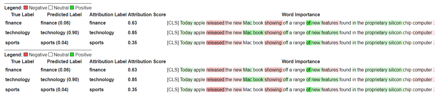
让我们从初始化变形金刚的问题答案模型和令牌的开始,然后通过QuestionAnsweringExplainer运行它。
在此示例中,我们使用的是bert-large-uncased-whole-word-masking-finetuned-squad ,这是一个在小队上进行的BERT模型。
 from transformers import AutoModelForQuestionAnswering , AutoTokenizer
from transformers_interpret import QuestionAnsweringExplainer

tokenizer = AutoTokenizer . from_pretrained ( "bert-large-uncased-whole-word-masking-finetuned-squad" )
model = AutoModelForQuestionAnswering . from_pretrained ( "bert-large-uncased-whole-word-masking-finetuned-squad" )

qa_explainer = QuestionAnsweringExplainer (
    model ,
    tokenizer ,
)

context = """
In Artificial Intelligence and machine learning, Natural Language Processing relates to the usage of machines to process and understand human language.
Many researchers currently work in this space.
"""

word_attributions = qa_explainer (
    "What is natural language processing ?" ,
    context ,
)
这将返回以下内容,其中包含词语属性,用于答案的预测启动和结束位置。
 > >> word_attributions
{ 'start' : [( '[CLS]' , 0.0 ),
  ( 'what' , 0.9177170660377296 ),
  ( 'is' , 0.13382234898765258 ),
  ( 'natural' , 0.08061747350142005 ),
  ( 'language' , 0.013138062762511409 ),
  ( 'processing' , 0.11135923869816286 ),
  ( '?' , 0.00858057388924361 ),
  ( '[SEP]' , - 0.09646373141894966 ),
  ( 'in' , 0.01545633993975799 ),
  ( 'artificial' , 0.0472082598707737 ),
  ( 'intelligence' , 0.026687249355110867 ),
  ( 'and' , 0.01675371260058537 ),
  ( 'machine' , - 0.08429502436554961 ),
  ( 'learning' , 0.0044827685126163355 ),
  ( ',' , - 0.02401013152520878 ),
  ( 'natural' , - 0.0016756080249823537 ),
  ( 'language' , 0.0026815068421401885 ),
  ( 'processing' , 0.06773157580722854 ),
  ( 'relates' , 0.03884601576992908 ),
  ( 'to' , 0.009783797821526368 ),
  ( 'the' , - 0.026650922910540952 ),
  ( 'usage' , - 0.010675019721821147 ),
  ( 'of' , 0.015346787885898537 ),
  ( 'machines' , - 0.08278008270160107 ),
  ( 'to' , 0.12861387892768839 ),
  ( 'process' , 0.19540146386642743 ),
  ( 'and' , 0.009942879959615826 ),
  ( 'understand' , 0.006836894853320319 ),
  ( 'human' , 0.05020451122579102 ),
  ( 'language' , - 0.012980795199301 ),
  ( '.' , 0.00804358248127772 ),
  ( 'many' , 0.02259009321498161 ),
  ( 'researchers' , - 0.02351650942555469 ),
  ( 'currently' , 0.04484573078852946 ),
  ( 'work' , 0.00990399948294476 ),
  ( 'in' , 0.01806961211334615 ),
  ( 'this' , 0.13075899776164499 ),
  ( 'space' , 0.004298315347838973 ),
  ( '.' , - 0.003767904539347979 ),
  ( '[SEP]' , - 0.08891544093454595 )],
 'end' : [( '[CLS]' , 0.0 ),
  ( 'what' , 0.8227231947501547 ),
  ( 'is' , 0.0586864942952253 ),
  ( 'natural' , 0.0938903563379123 ),
  ( 'language' , 0.058596976016400674 ),
  ( 'processing' , 0.1632374290269829 ),
  ( '?' , 0.09695686057123237 ),
  ( '[SEP]' , - 0.11644447033554006 ),
  ( 'in' , - 0.03769172371919206 ),
  ( 'artificial' , 0.06736158404049886 ),
  ( 'intelligence' , 0.02496399001288386 ),
  ( 'and' , - 0.03526028847762427 ),
  ( 'machine' , - 0.20846431491771975 ),
  ( 'learning' , 0.00904892847529654 ),
  ( ',' , - 0.02949905488474854 ),
  ( 'natural' , 0.011024507784743872 ),
  ( 'language' , 0.0870741751282507 ),
  ( 'processing' , 0.11482449622317169 ),
  ( 'relates' , 0.05008962090922852 ),
  ( 'to' , 0.04079118393166258 ),
  ( 'the' , - 0.005069048880616451 ),
  ( 'usage' , - 0.011992752445836278 ),
  ( 'of' , 0.01715183316135495 ),
  ( 'machines' , - 0.29823535624026265 ),
  ( 'to' , - 0.0043760160855057925 ),
  ( 'process' , 0.10503217484645223 ),
  ( 'and' , 0.06840313586976698 ),
  ( 'understand' , 0.057184000619403944 ),
  ( 'human' , 0.0976805947708315 ),
  ( 'language' , 0.07031163646606695 ),
  ( '.' , 0.10494566513897102 ),
  ( 'many' , 0.019227154676079487 ),
  ( 'researchers' , - 0.038173913797800885 ),
  ( 'currently' , 0.03916641120002003 ),
  ( 'work' , 0.03705371672439422 ),
  ( 'in' , - 0.0003155975107591203 ),
  ( 'this' , 0.17254932354022232 ),
  ( 'space' , 0.0014311439625599323 ),
  ( '.' , 0.060637932829867736 ),
  ( '[SEP]' , - 0.09186286505530596 )]}
我们可以通过以下方式获得预测答案的文本跨度:
 > >> qa_explainer . predicted_answer
'usage of machines to process and understand human language' 对于QuestionAnsweringExplainer ,可视化方法()方法返回带有两个行的表。第一行代表答案的开始位置的属性,第二行代表答案的终端位置的属性。
qa_explainer . visualize ( "bert_qa_viz.html" )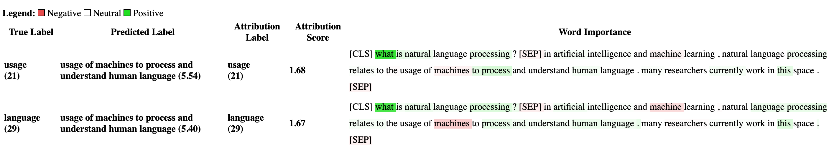
目前,这是一个正在积极开发的实验解释器,尚未进行全面测试。解释器的API与归因方法一样,如果找到任何错误,请告诉我。
让我们从初始化变形金刚的令牌类模型和令牌器,然后通过TokenClassificationExplainer运行它。
在此示例中,我们使用的是dslim/bert-base-NER ,这是在Conll-2003上名为“实体识别数据集”上进行的BERT模型。
 from transformers import AutoModelForTokenClassification , AutoTokenizer
from transformers_interpret import TokenClassificationExplainer

model = AutoModelForTokenClassification . from_pretrained ( 'dslim/bert-base-NER' )
tokenizer = AutoTokenizer . from_pretrained ( 'dslim/bert-base-NER' )

ner_explainer = TokenClassificationExplainer (
    model ,
    tokenizer ,
)

sample_text = "We visited Paris last weekend, where Emmanuel Macron lives."

word_attributions = ner_explainer ( sample_text , ignored_labels = [ 'O' ])为了减少计算的属性数量,我们告诉解释器忽略了标记的令牌,其预测标签为'O' 。我们还可以告诉解释器忽略某些索引,以提供列表作为参数ignored_indexes参数。
它将返回以下命令,其中包括预测标签和每个令牌的归因,除了被预测为“ O”的标签:
 > >> word_attributions
{ 'paris' : { 'label' : 'B-LOC' ,
  'attribution_scores' : [( '[CLS]' , 0.0 ),
   ( 'we' , - 0.014352325471387907 ),
   ( 'visited' , 0.32915222186559123 ),
   ( 'paris' , 0.9086791784795596 ),
   ( 'last' , 0.15181203147624034 ),
   ( 'weekend' , 0.14400210630677038 ),
   ( ',' , 0.01899744327012935 ),
   ( 'where' , - 0.039402005463239465 ),
   ( 'emmanuel' , 0.061095284002642025 ),
   ( 'macro' , 0.004192922551105228 ),
   ( '##n' , 0.09446355513057757 ),
   ( 'lives' , - 0.028724312616455003 ),
   ( '.' , 0.08099007392937585 ),
   ( '[SEP]' , 0.0 )]},
 'emmanuel' : { 'label' : 'B-PER' ,
  'attribution_scores' : [( '[CLS]' , 0.0 ),
   ( 'we' , - 0.006933030636686712 ),
   ( 'visited' , 0.10396962390436904 ),
   ( 'paris' , 0.14540758744233165 ),
   ( 'last' , 0.08024018944451371 ),
   ( 'weekend' , 0.10687970996804418 ),
   ( ',' , 0.1793198466387937 ),
   ( 'where' , 0.3436407835483767 ),
   ( 'emmanuel' , 0.8774892642652167 ),
   ( 'macro' , 0.03559399361048316 ),
   ( '##n' , 0.1516315604785551 ),
   ( 'lives' , 0.07056441327498127 ),
   ( '.' , - 0.025820924624605487 ),
   ( '[SEP]' , 0.0 )]},
 'macro' : { 'label' : 'I-PER' ,
  'attribution_scores' : [( '[CLS]' , 0.0 ),
   ( 'we' , 0.05578067326280157 ),
   ( 'visited' , 0.00857021283406586 ),
   ( 'paris' , 0.16559056506114297 ),
   ( 'last' , 0.08285256685903823 ),
   ( 'weekend' , 0.10468727443796395 ),
   ( ',' , 0.09949509071515888 ),
   ( 'where' , 0.3642458274356929 ),
   ( 'emmanuel' , 0.7449335213978788 ),
   ( 'macro' , 0.3794625659183485 ),
   ( '##n' , - 0.2599031433800762 ),
   ( 'lives' , 0.20563450682196147 ),
   ( '.' , - 0.015607017319486929 ),
   ( '[SEP]' , 0.0 )]},
 '##n' : { 'label' : 'I-PER' ,
  'attribution_scores' : [( '[CLS]' , 0.0 ),
   ( 'we' , 0.025194121717285252 ),
   ( 'visited' , - 0.007415022865239864 ),
   ( 'paris' , 0.09478357303107598 ),
   ( 'last' , 0.06927939834474463 ),
   ( 'weekend' , 0.0672008033510708 ),
   ( ',' , 0.08316907214363504 ),
   ( 'where' , 0.3784915854680165 ),
   ( 'emmanuel' , 0.7729352621546081 ),
   ( 'macro' , 0.4148652759139777 ),
   ( '##n' , - 0.20853534512145033 ),
   ( 'lives' , 0.09445057087678274 ),
   ( '.' , - 0.094274985907366 ),
   ( '[SEP]' , 0.0 )]},
 '[SEP]' : { 'label' : 'B-LOC' ,
  'attribution_scores' : [( '[CLS]' , 0.0 ),
   ( 'we' , - 0.3694351403796742 ),
   ( 'visited' , 0.1699038407402483 ),
   ( 'paris' , 0.5461587414992369 ),
   ( 'last' , 0.0037948102770307517 ),
   ( 'weekend' , 0.1628100955702496 ),
   ( ',' , 0.4513093410909263 ),
   ( 'where' , - 0.09577409464161038 ),
   ( 'emmanuel' , 0.48499459835388914 ),
   ( 'macro' , - 0.13528905587653023 ),
   ( '##n' , 0.14362969934754344 ),
   ( 'lives' , - 0.05758007024257254 ),
   ( '.' , - 0.13970977266152554 ),
( '[SEP]' , 0.0 )]}}对于TokenClassificationExplainer开发器,可视化方法()方法返回具有与令牌一样多的行的表。
ner_explainer . visualize ( "bert_ner_viz.html" )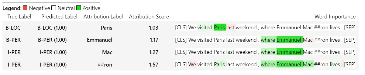
有关TokenClassificationExplainer工作方式的更多详细信息,您可以查看笔记本电脑/ner_example.ipynb。
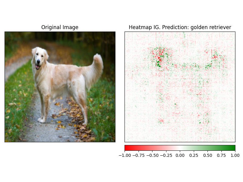
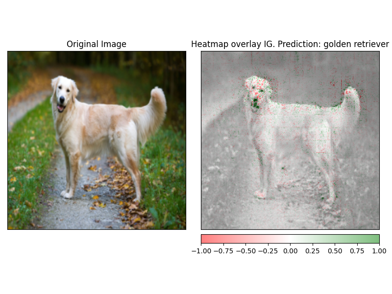
ImageClassificationExplainer旨在与经过训练用于图像分类(SWIN,VIT等)的所有模型一起使用。它为该图像中的每个像素提供了归因,可以使用visualize方法中内置的解释器轻松可视化。
初始化图像分类非常简单,您所需要的只是图像分类模型固定或培训,可与HuggingFace及其特征提取器一起使用。
在此示例中,我们使用的是google/vit-base-patch16-224 ,这是在Imagenet-21K上预先训练的视觉变压器(VIT)模型,可预测1000个可能的类别。
 from transformers import AutoFeatureExtractor , AutoModelForImageClassification
from transformers_interpret import ImageClassificationExplainer
from PIL import Image
import requests

model_name = "google/vit-base-patch16-224"
model = AutoModelForImageClassification . from_pretrained ( model_name )
feature_extractor = AutoFeatureExtractor . from_pretrained ( model_name )

# With both the model and feature extractor initialized we are now able to get explanations on an image, we will use a simple image of a golden retriever.
image_link = "https://imagesvc.meredithcorp.io/v3/mm/image?url=https%3A%2F%2Fstatic.onecms.io%2Fwp-content%2Fuploads%2Fsites%2F47%2F2020%2F08%2F16%2Fgolden-retriever-177213599-2000.jpg"

image = Image . open ( requests . get ( image_link , stream = True ). raw )

image_classification_explainer = ImageClassificationExplainer ( model = model , feature_extractor = feature_extractor )

image_attributions = image_classification_explainer (
    image
)

print ( image_attributions . shape )
哪个将返回以下单元列表:
> >> torch . Size ([ 1 , 3 , 224 , 224 ])因为我们正在处理图像的可视化比文本模型更简单。
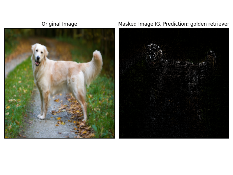
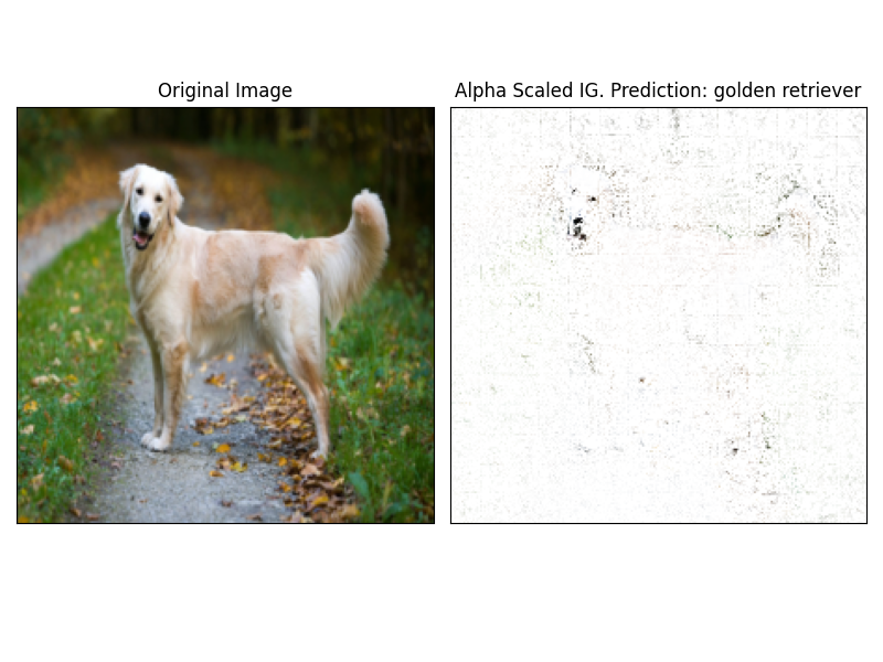
使用解释器的visualize方法可以轻松地可视化attrbution。当前有4种支持的可视化方法。
heatmap - 使用图像的尺寸绘制正归因和负归因的热图。overlay - 热图被覆盖在原始图像的灰度版本上masked_image属性的绝对值用于通过原始图像创建掩码alpha_scaling将每个像素的Alpha通道(透明度)设置为等于归一化的归因值。 image_classification_explainer . visualize (
method = "heatmap" ,
side_by_side = True ,
outlier_threshold = 0.03
)
 image_classification_explainer . visualize (
    method = "overlay" ,
    side_by_side = True ,
    outlier_threshold = 0.03

)
 image_classification_explainer . visualize (
    method = "masked_image" ,
    side_by_side = True ,
    outlier_threshold = 0.03

)
 image_classification_explainer . visualize (
    method = "alpha_scaling" ,
    side_by_side = True ,
    outlier_threshold = 0.03

)
该软件包仍在积极开发中,并且有更多计划。对于1.0.0版本,我们的目标是:
如果您想做出贡献,请查看我们的贡献指南
该存储库的维护者是@cdpierse。
如果您有任何疑问,建议或想做出贡献(请这样做?),请随时通过[email protected]与您取得联系。
如果您发现模型的解释性和解释性有趣,我也强烈建议您检查Captum。
该包裹坐落在Pytorch Captum和拥抱脸的团队所做的令人难以置信的工作的肩膀上,如果不是因为他们在ML和模型可解释性领域所做的出色工作,就不存在。
该软件包中的所有属性都是使用Pytorch的解释性软件包CAPTUM计算的。有关与Captum相关的一些有用链接,请参见下文。
集成梯度(IG)和IT层集成梯度(LIG)的变化是当前构建变压器解释的核心归因方法。以下是一些有用的资源,包括原始论文和一些视频链接,解释了内部力学。如果您对变形金刚内部发生的事情感到好奇,我强烈建议您查看至少其中一种资源。
Captum链接
以下是我用来帮助我使用Captum将此包装在一起的一些链接。感谢@davidefiocco的洞察力。


