YOLOv4 pytorch
1.0.0
Conseils: 深度学习指导 , 目标检测、目标跟踪、语义分割等 , 小型数据集详询 QQ3419923783
| nom | ensemble de données de train | ensemble de données de test | taille de test | carte | Temps d'inférence (MS) | paramètres (m) | lien de modèle |
|---|---|---|---|---|---|---|---|
| mobilenetv2-yolov4 | VOC Trainval (07 + 12) | Test de COV (07) | 416 | 0,851 | 11.29 | 46.34 | args |
MobileNetv3-Yolov4 arrive! (Vous n'avez qu'à modifier le modèle_type dans config / yolov4_config.py)
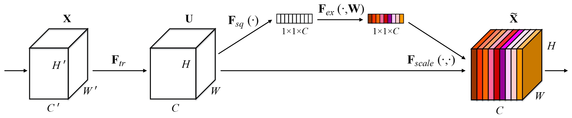
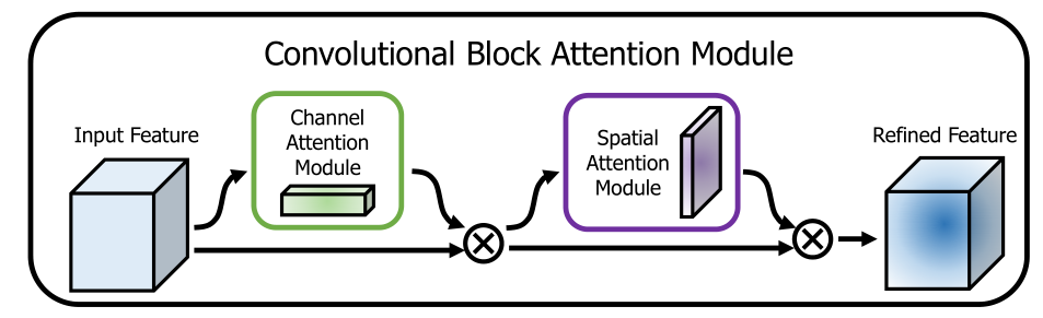
Ce repo ajoute quelques méthodes d'attention utiles dans le squelette. Les images suivantes illustrent une telle chose:
Ce repo est simple à utiliser, facile à lire et simple à améliorer par rapport aux autres !!!
Exécutez le script d'installation pour installer toutes les dépendances. Vous devez fournir le chemin d'installation conda (par exemple ~ / anaconda3) et le nom de l'environnement conda créé (ici YOLOv4-pytorch ).
pip3 install -r requirements.txt --userRemarque: Le script d'installation a été testé sur un système Ubuntu 18.04 et Window 10. En cas de problèmes, vérifiez les instructions d'installation détaillées.
git clone github.com/argusswift/YOLOv4-pytorch.git Mettez à jour le "PROJECT_PATH" dans la config / yolov4_config.py.
 # Download the data.
cd $HOME /data
wget http://host.robots.ox.ac.uk/pascal/VOC/voc2012/VOCtrainval_11-May-2012.tar
wget http://host.robots.ox.ac.uk/pascal/VOC/voc2007/VOCtrainval_06-Nov-2007.tar
wget http://host.robots.ox.ac.uk/pascal/VOC/voc2007/VOCtest_06-Nov-2007.tar
# Extract the data.
tar -xvf VOCtrainval_11-May-2012.tar
tar -xvf VOCtrainval_06-Nov-2007.tar
tar -xvf VOCtest_06-Nov-2007.tar # step1: download the following data and annotation
2017 Train images [118K/18GB]
2017 Val images [5K/1GB]
2017 Test images [41K/6GB]
2017 Train/Val annotations [241MB]
# step2: arrange the data to the following structure
COCO
---train
---test
---val
---annotations"DATA_PATH" dans la config / yolov4_config.py.weight/ dans le Yolov4 et mettez le fichier de poids. Exécutez la commande suivante pour démarrer la formation et voir les détails de la config/yolov4_config.py et vous devez définir Data_type est VOC ou CoCo lorsque vous exécutez le programme de formation.
CUDA_VISIBLE_DEVICES=0 nohup python -u train.py --weight_path weight/yolov4.weights --gpu_id 0 > nohup.log 2>&1 & Aussi * il prend en charge la repreuve de la formation en ajoutant --resume , il se chargera last.pt automatiquement en utilisant des commotions
CUDA_VISIBLE_DEVICES=0 nohup python -u train.py --weight_path weight/last.pt --gpu_id 0 > nohup.log 2>&1 & Modifiez votre chemin IMG de détection: data_test = / path / to / votre / test_data # vos propres images
for VOC dataset:
CUDA_VISIBLE_DEVICES=0 python3 eval_voc.py --weight_path weight/best.pt --gpu_id 0 --visiual $DATA_TEST --eval --mode det
for COCO dataset:
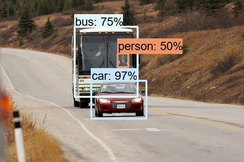
CUDA_VISIBLE_DEVICES=0 python3 eval_coco.py --weight_path weight/best.pt --gpu_id 0 --visiual $DATA_TEST --eval --mode det Les images peuvent être vues dans la output/ . Vous pouvez voir des photos comme suit:
Modifier:
CUDA_VISIBLE_DEVICES=0 python3 video_test.py --weight_path best.pt --gpu_id 0 --video_path video.mp4 --output_dir --output_dirModifiez votre jeu de données d'évaluation: data_path = / path / to / votre / test_data # vos propres images
 for VOC dataset:
CUDA_VISIBLE_DEVICES=0 python3 eval_voc.py --weight_path weight/best.pt --gpu_id 0 --visiual $DATA_TEST --eval --mode val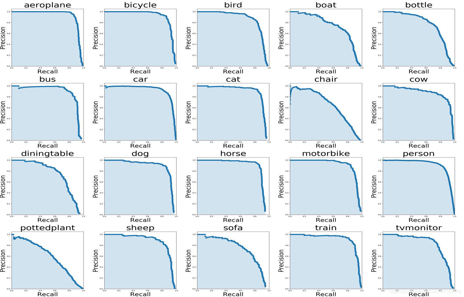
Si vous souhaitez voir l'image ci-dessus, vous devez utiliser les commandes Suivre:
 # To get ground truths of your dataset
python3 utils/get_gt_txt.py
# To plot P-R curve and calculate mean average precision
python3 utils/get_map.py Modifiez votre jeu de données d'évaluation: data_path = / path / to / votre / test_data # vos propres images
CUDA_VISIBLE_DEVICES=0 python3 eval_coco.py --weight_path weight/best.pt --gpu_id 0 --visiual $DATA_TEST --eval --mode val

type=bbox
Running per image evaluation...      DONE (t=0.34s).
Accumulating evaluation results...   DONE (t=0.08s).
 Average Precision  (AP) @[ IoU = 0.50:0.95 | area =   all | maxDets = 100 ] = 0.438
 Average Precision  (AP) @[ IoU = 0.50      | area =   all | maxDets = 100 ] = 0.607
 Average Precision  (AP) @[ IoU = 0.75      | area =   all | maxDets = 100 ] = 0.469
 Average Precision  (AP) @[ IoU = 0.50:0.95 | area = small | maxDets = 100 ] = 0.253
 Average Precision  (AP) @[ IoU = 0.50:0.95 | area = medium | maxDets = 100 ] = 0.486
 Average Precision  (AP) @[ IoU = 0.50:0.95 | area = large | maxDets = 100 ] = 0.567
 Average Recall     (AR) @[ IoU = 0.50:0.95 | area =   all | maxDets =  1 ] = 0.342
 Average Recall     (AR) @[ IoU = 0.50:0.95 | area =   all | maxDets = 10 ] = 0.571
 Average Recall     (AR) @[ IoU = 0.50:0.95 | area =   all | maxDets = 100 ] = 0.632
 Average Recall     (AR) @[ IoU = 0.50:0.95 | area = small | maxDets = 100 ] = 0.458
 Average Recall     (AR) @[ IoU = 0.50:0.95 | area = medium | maxDets = 100 ] = 0.691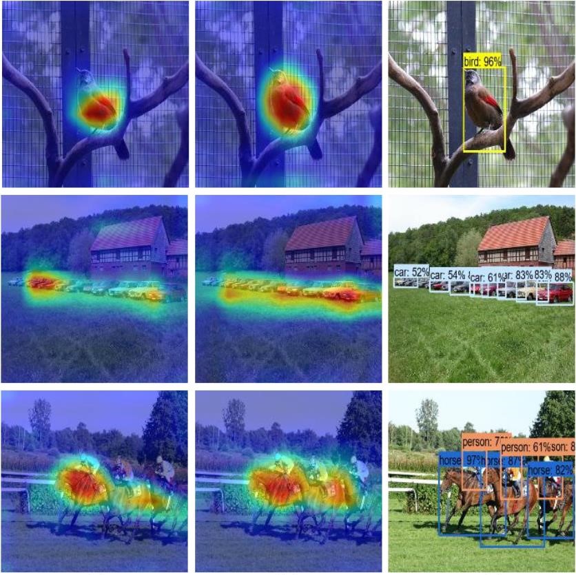
Average Recall (AR) @[ IoU = 0.50:0.95 | area = large | maxDets = 100 ] = 0.790python3 utils/modelsize.pySet showatt = ture dans val_voc.py et vous verrez les marques de chaleur émergées de la sortie du réseau
 for VOC dataset:
CUDA_VISIBLE_DEVICES=0 python3 eval_voc.py --weight_path weight/best.pt --gpu_id 0 --visiual $DATA_TEST --eval
for COCO dataset:
CUDA_VISIBLE_DEVICES=0 python3 eval_coco.py --weight_path weight/best.pt --gpu_id 0 --visiual $DATA_TEST --eval
Les thermaps peuvent être vus dans la output/ comme ceci: