YOLOv4 pytorch
1.0.0
Consejos: 深度学习指导 , 目标检测、目标跟踪、语义分割等 小型数据集详询 小型数据集详询 QQ3419923783
| nombre | conjunto de datos de tren | conjunto de datos de prueba | tamaño de prueba | mapa | Tiempo de inferencia (MS) | parámetros (m) | enlace modelo |
|---|---|---|---|---|---|---|---|
| mobilenetv2-yolov4 | VOC Trainval (07+12) | Prueba de VOC (07) | 416 | 0.851 | 11.29 | 46.34 | argumentos |
¡MobileNetv3-yolov4 está llegando! (Solo necesita cambiar el model_type en config/yolov4_config.py)
Este repositorio agrega algunos métodos de atención útiles en la columna vertebral. Las siguientes imágenes ilustran tal cosa:
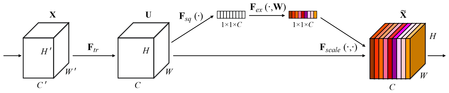
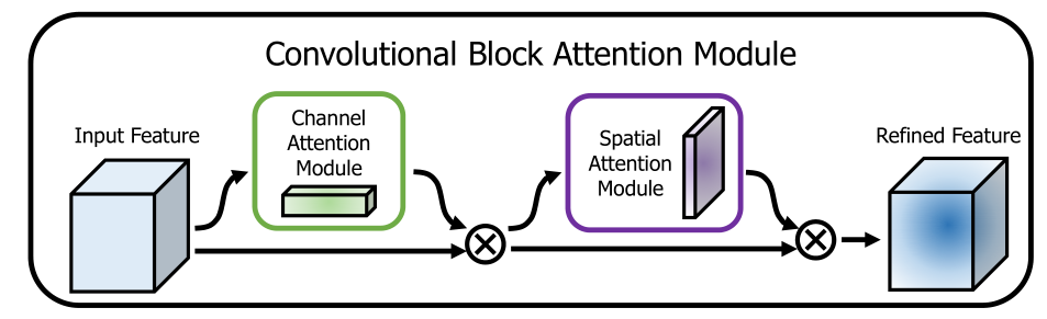
¡Este repositorio es fácil de usar, fácil de leer y sin complicaciones para mejorar en comparación con los demás!
Ejecute el script de instalación para instalar todas las dependencias. Debe proporcionar la ruta de instalación de Conda (por ejemplo, anaconda3) y el nombre del entorno de conda creado (aquí YOLOv4-pytorch ).
pip3 install -r requirements.txt --userNota: El script de instalación se ha probado en un sistema Ubuntu 18.04 y Window 10. En caso de problemas, verifique las instrucciones de instalación detalladas.
git clone github.com/argusswift/YOLOv4-pytorch.git Actualice el "PROJECT_PATH" en config/yolov4_config.py.
 # Download the data.
cd $HOME /data
wget http://host.robots.ox.ac.uk/pascal/VOC/voc2012/VOCtrainval_11-May-2012.tar
wget http://host.robots.ox.ac.uk/pascal/VOC/voc2007/VOCtrainval_06-Nov-2007.tar
wget http://host.robots.ox.ac.uk/pascal/VOC/voc2007/VOCtest_06-Nov-2007.tar
# Extract the data.
tar -xvf VOCtrainval_11-May-2012.tar
tar -xvf VOCtrainval_06-Nov-2007.tar
tar -xvf VOCtest_06-Nov-2007.tar # step1: download the following data and annotation
2017 Train images [118K/18GB]
2017 Val images [5K/1GB]
2017 Test images [41K/6GB]
2017 Train/Val annotations [241MB]
# step2: arrange the data to the following structure
COCO
---train
---test
---val
---annotations"DATA_PATH" en el config/yolov4_config.py.weight/ en el Yolov4 y coloque el archivo de peso. Ejecute el siguiente comando para comenzar la capacitación y vea los detalles en config/yolov4_config.py y debe establecer data_type es VOC o COCO cuando ejecuta el programa de entrenamiento.
CUDA_VISIBLE_DEVICES=0 nohup python -u train.py --weight_path weight/yolov4.weights --gpu_id 0 > nohup.log 2>&1 & También * admite reanudar la capacitación agregando --resume , se cargará last.pt .
CUDA_VISIBLE_DEVICES=0 nohup python -u train.py --weight_path weight/last.pt --gpu_id 0 > nohup.log 2>&1 & Modifique su ruta Detecte IMG: data_test =/path/to/su/test_data # sus propias imágenes
for VOC dataset:
CUDA_VISIBLE_DEVICES=0 python3 eval_voc.py --weight_path weight/best.pt --gpu_id 0 --visiual $DATA_TEST --eval --mode det
for COCO dataset:
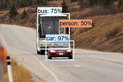
CUDA_VISIBLE_DEVICES=0 python3 eval_coco.py --weight_path weight/best.pt --gpu_id 0 --visiual $DATA_TEST --eval --mode det Las imágenes se pueden ver en la output/ . Podrías ver fotos como sigue:
Modificar:
CUDA_VISIBLE_DEVICES=0 python3 video_test.py --weight_path best.pt --gpu_id 0 --video_path video.mp4 --output_dir --output_dirModifique su ruta de conjunto de datos de evaluación: data_path =/path/to/su/test_data # sus propias imágenes
 for VOC dataset:
CUDA_VISIBLE_DEVICES=0 python3 eval_voc.py --weight_path weight/best.pt --gpu_id 0 --visiual $DATA_TEST --eval --mode val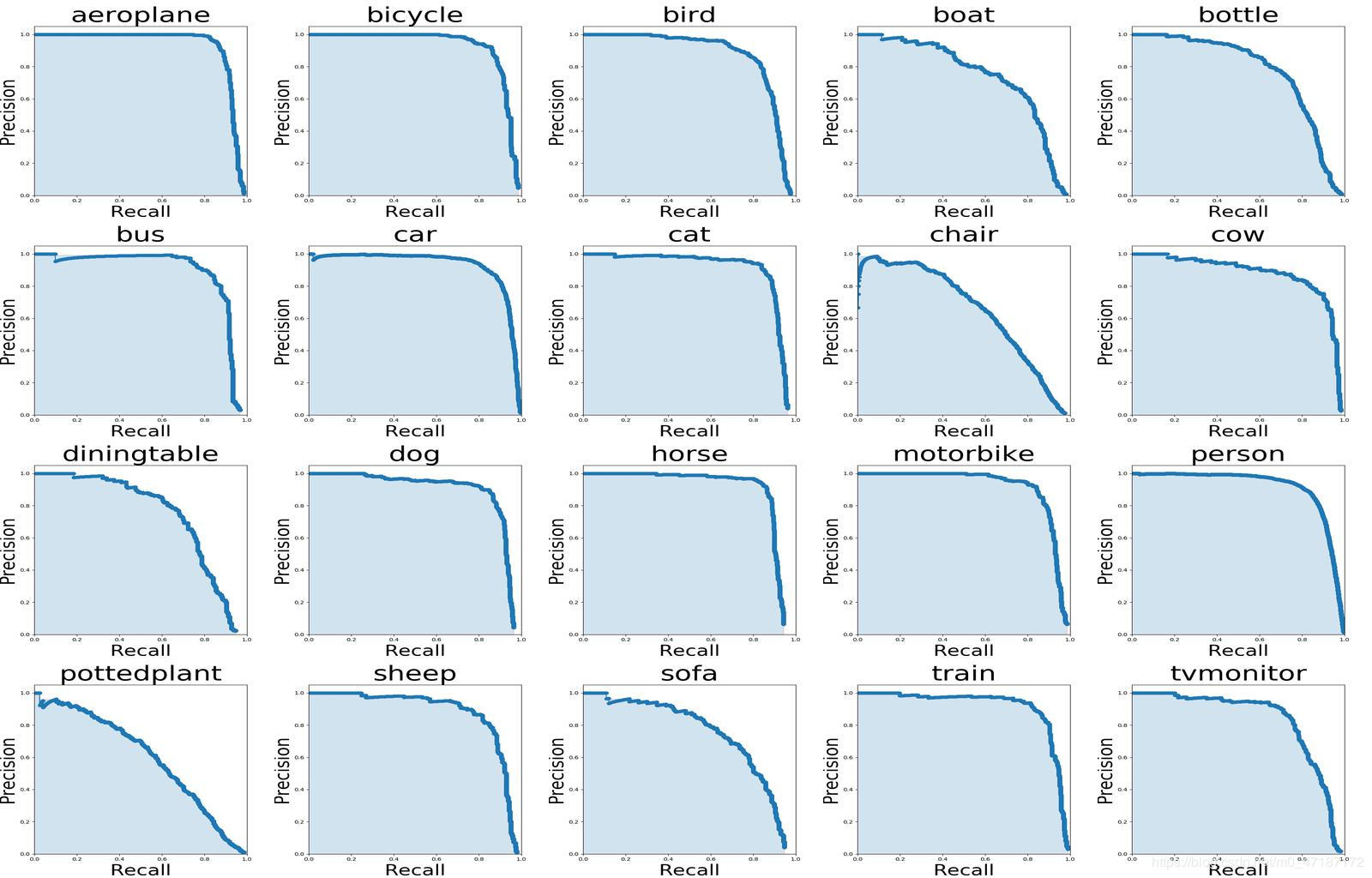
Si desea ver la imagen de arriba, debe usar comandos de seguimiento:
 # To get ground truths of your dataset
python3 utils/get_gt_txt.py
# To plot P-R curve and calculate mean average precision
python3 utils/get_map.py Modifique su ruta de conjunto de datos de evaluación: data_path =/path/to/su/test_data # sus propias imágenes
CUDA_VISIBLE_DEVICES=0 python3 eval_coco.py --weight_path weight/best.pt --gpu_id 0 --visiual $DATA_TEST --eval --mode val

type=bbox
Running per image evaluation...      DONE (t=0.34s).
Accumulating evaluation results...   DONE (t=0.08s).
 Average Precision  (AP) @[ IoU = 0.50:0.95 | area =   all | maxDets = 100 ] = 0.438
 Average Precision  (AP) @[ IoU = 0.50      | area =   all | maxDets = 100 ] = 0.607
 Average Precision  (AP) @[ IoU = 0.75      | area =   all | maxDets = 100 ] = 0.469
 Average Precision  (AP) @[ IoU = 0.50:0.95 | area = small | maxDets = 100 ] = 0.253
 Average Precision  (AP) @[ IoU = 0.50:0.95 | area = medium | maxDets = 100 ] = 0.486
 Average Precision  (AP) @[ IoU = 0.50:0.95 | area = large | maxDets = 100 ] = 0.567
 Average Recall     (AR) @[ IoU = 0.50:0.95 | area =   all | maxDets =  1 ] = 0.342
 Average Recall     (AR) @[ IoU = 0.50:0.95 | area =   all | maxDets = 10 ] = 0.571
 Average Recall     (AR) @[ IoU = 0.50:0.95 | area =   all | maxDets = 100 ] = 0.632
 Average Recall     (AR) @[ IoU = 0.50:0.95 | area = small | maxDets = 100 ] = 0.458
 Average Recall     (AR) @[ IoU = 0.50:0.95 | area = medium | maxDets = 100 ] = 0.691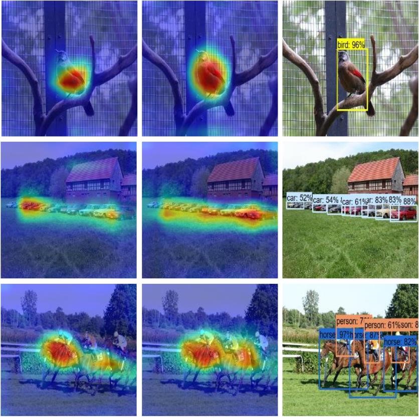
Average Recall (AR) @[ IoU = 0.50:0.95 | area = large | maxDets = 100 ] = 0.790python3 utils/modelsize.pyEstablecer showatt = ture en val_voc.py y verá que los mapas de calor surgen de la salida de la red '
 for VOC dataset:
CUDA_VISIBLE_DEVICES=0 python3 eval_voc.py --weight_path weight/best.pt --gpu_id 0 --visiual $DATA_TEST --eval
for COCO dataset:
CUDA_VISIBLE_DEVICES=0 python3 eval_coco.py --weight_path weight/best.pt --gpu_id 0 --visiual $DATA_TEST --eval
Los mapas de calor se pueden ver en la output/ así: