skpr
v1.7.0
SKPR est une conception open source de Suite Experiments pour générer et évaluer des conceptions optimales dans R. Voici un échantillon de ce que SKPR offre:
 # To install:
install.packages( " skpr " )

# To install the latest version from Github:
# install.packages("devtools")
devtools :: install_github( " tylermorganwall/skpr " )gen_design() génère des conceptions optimales à partir d'un ensemble de candidats, étant donné un modèle et le nombre souhaité de cycles.eval_design() évalue la puissance paramétrique pour les modèles linéaires, pour les conceptions normales et divisées.eval_design_mc() évalue la puissance avec une simulation Monte Carlo, pour les modèles linéaires linéaires et généralisés. Cette fonction prend également en charge le calcul de la puissance pour les conceptions de places fendues à l'aide de REML.eval_design_survival_mc() Évalue la puissance avec une simulation Monte Carlo, permettant à l'utilisateur de spécifier un point auquel les données sont censurées.eval_design_custom_mc() permet à l'utilisateur d'importer ses propres bibliothèques et d'utiliser le cadre Monte Carlo fourni par SKPR pour calculer la puissance.calculate_power_curves() fournit une interface pour automatiser la génération et l'évaluation des conceptions pour créer des courbes de taille et de taille de la taille de l'échantillon et de l'échantillon.skprGUI() ouvre l'interface graphique dans rstudio ou un navigateur externe.Si en plus, le package propose deux fonctions pour générer des tracés communs liés aux conceptions:
plot_correlations() génère une carte couleur des corrélations entre les variables.plot_fds() génère la fraction du tracé de l'espace de conception pour une conception donnée.## skprgui
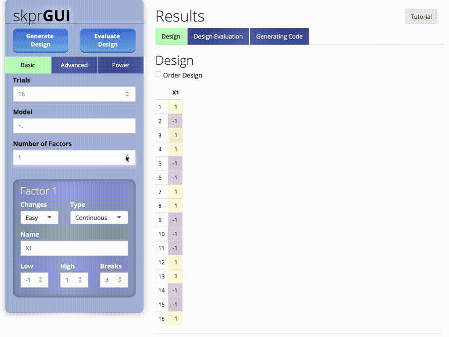
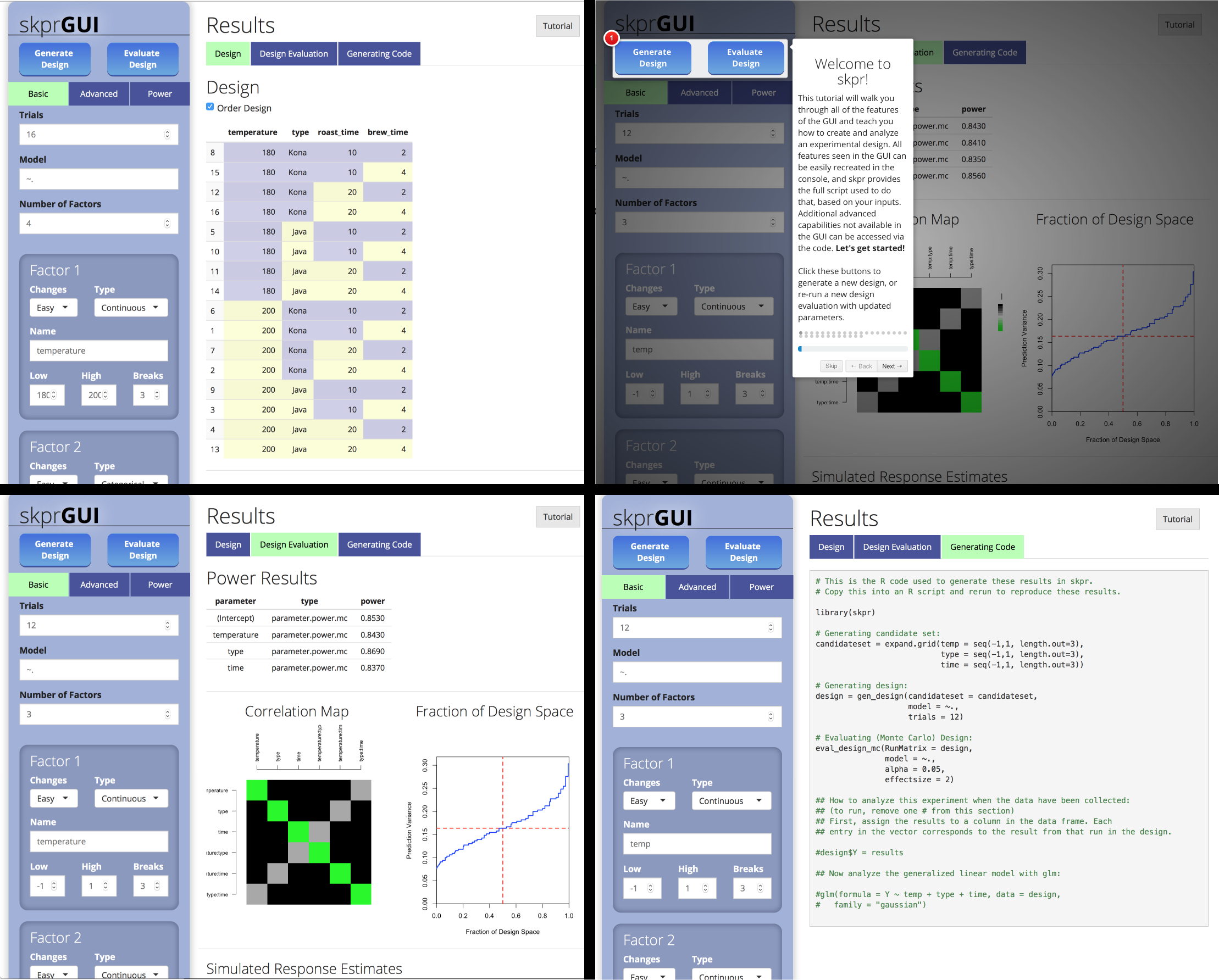
skprGUI() fournit une interface utilisateur graphique pour accéder à toutes les principales fonctionnalités de SKPR. Un tutoriel interactif est fourni pour familiariser l'utilisateur avec les fonctionnalités disponibles. Tapez skprGUI() pour commencer. Captures d'écran:
library( skpr )

# Generate a candidate set of all potential design points to be considered in the experiment
# The hypothetical experiment is determining what affects the caffeine content in coffee
candidate_set = expand.grid( temp = c( 80 , 90 , 100 ),
                            type = c( " Kona " , " Java " ),
                            beansize = c( " Large " , " Medium " , " Small " ))
candidate_set
# >    temp type beansize
# > 1    80 Kona    Large
# > 2    90 Kona    Large
# > 3   100 Kona    Large
# > 4    80 Java    Large
# > 5    90 Java    Large
# > 6   100 Java    Large
# > 7    80 Kona   Medium
# > 8    90 Kona   Medium
# > 9   100 Kona   Medium
# > 10   80 Java   Medium
# > 11   90 Java   Medium
# > 12  100 Java   Medium
# > 13   80 Kona    Small
# > 14   90 Kona    Small
# > 15  100 Kona    Small
# > 16   80 Java    Small
# > 17   90 Java    Small
# > 18  100 Java    Small

# Generate the design (default D-optimal)
design = gen_design( candidateset = candidate_set ,
                    model = ~ temp + type + beansize ,
                    trials = 12 )
design
# >    temp type beansize
# > 1    80 Java   Medium
# > 2   100 Java    Large
# > 3   100 Java    Small
# > 4    80 Java    Large
# > 5    80 Kona   Medium
# > 6    80 Kona    Small
# > 7   100 Kona    Small
# > 8   100 Kona   Medium
# > 9    80 Kona    Large
# > 10  100 Java   Medium
# > 11  100 Kona    Large
# > 12   80 Java    Small

# Evaluate power for the design with an allowable type-I error of 5% (default)
eval_design( design )
# >     parameter            type     power
# > 1 (Intercept)    effect.power 0.8424665
# > 2        temp    effect.power 0.8424665
# > 3        type    effect.power 0.8424665
# > 4    beansize    effect.power 0.5165386
# > 5 (Intercept) parameter.power 0.8424665
# > 6        temp parameter.power 0.8424665
# > 7       type1 parameter.power 0.8424665
# > 8   beansize1 parameter.power 0.5593966
# > 9   beansize2 parameter.power 0.5593966
# > ============Evaluation Info============
# > * Alpha = 0.05 * Trials = 12 * Blocked = FALSE
# > * Evaluating Model = ~temp + type + beansize
# > * Anticipated Coefficients = c(1, 1, 1, 1, -1)
# > * Contrasts = `contr.sum`
# > * Parameter Analysis Method = `lm(...)`
# > * Effect Analysis Method = `car::Anova(fit, type = "III")`

# Evaluate power for the design using a Monte Carlo simulation.
# Here, we set the effect size (here, the signal-to-noise ratio) to 1.5.
eval_design_mc( design , effectsize = 1.5 )
# >     parameter               type power
# > 1 (Intercept)    effect.power.mc 0.600
# > 2        temp    effect.power.mc 0.612
# > 3        type    effect.power.mc 0.610
# > 4    beansize    effect.power.mc 0.316
# > 5 (Intercept) parameter.power.mc 0.600
# > 6        temp parameter.power.mc 0.612
# > 7       type1 parameter.power.mc 0.610
# > 8   beansize1 parameter.power.mc 0.359
# > 9   beansize2 parameter.power.mc 0.354
# > ===========Evaluation Info============
# > * Alpha = 0.05 * Trials = 12 * Blocked = FALSE
# > * Evaluating Model = ~temp + type + beansize
# > * Anticipated Coefficients = c(0.750, 0.750, 0.750, 0.750, -0.750)
# > * Contrasts = `contr.sum`
# > * Parameter Analysis Method = `lm(...)`
# > * Effect Analysis Method = `car::Anova(fit, type = "III")`

# Evaluate power for the design using a Monte Carlo simulation, for a non-normal response.
# Here, we also increase the number of simululations to improve the precision of the results.
eval_design_mc( design , nsim = 5000 , glmfamily = " poisson " , effectsize = c( 2 , 6 ))
# >     parameter               type  power
# > 1 (Intercept)    effect.power.mc 0.9968
# > 2        temp    effect.power.mc 0.9826
# > 3        type    effect.power.mc 0.9832
# > 4    beansize    effect.power.mc 0.8502
# > 5 (Intercept) parameter.power.mc 0.9968
# > 6        temp parameter.power.mc 0.9826
# > 7       type1 parameter.power.mc 0.9832
# > 8   beansize1 parameter.power.mc 0.8842
# > 9   beansize2 parameter.power.mc 0.7052
# > ============Evaluation Info============
# > * Alpha = 0.05 * Trials = 12 * Blocked = FALSE
# > * Evaluating Model = ~temp + type + beansize
# > * Anticipated Coefficients = c(1.242, 0.549, 0.549, 0.549, -0.549)
# > * Contrasts = `contr.sum`
# > * Parameter Analysis Method = `glm(..., family = "poisson")`
# > * Effect Analysis Method = `car::Anova(fit, type = "III")`

# skpr was designed to operate with the pipe (|>) in mind.
# Here is an example of an entire design of experiments analysis in three lines:

expand.grid( temp = c( 80 , 90 , 100 ), type = c( " Kona " , " Java " ), beansize = c( " Large " , " Medium " , " Small " )) | >
  gen_design( model = ~ temp + type + beansize + beansize : type + I( temp ^ 2 ), trials = 24 , optimality = " I " ) | >
  eval_design_mc( detailedoutput = TRUE )
# >          parameter               type power anticoef alpha glmfamily trials
# > 1      (Intercept)    effect.power.mc 0.912       NA  0.05  gaussian     24
# > 2             temp    effect.power.mc 0.927       NA  0.05  gaussian     24
# > 3             type    effect.power.mc 0.997       NA  0.05  gaussian     24
# > 4         beansize    effect.power.mc 0.935       NA  0.05  gaussian     24
# > 5        I(temp^2)    effect.power.mc 0.637       NA  0.05  gaussian     24
# > 6    type:beansize    effect.power.mc 0.913       NA  0.05  gaussian     24
# > 7      (Intercept) parameter.power.mc 0.912        1  0.05  gaussian     24
# > 8             temp parameter.power.mc 0.927        1  0.05  gaussian     24
# > 9            type1 parameter.power.mc 0.997        1  0.05  gaussian     24
# > 10       beansize1 parameter.power.mc 0.917        1  0.05  gaussian     24
# > 11       beansize2 parameter.power.mc 0.913       -1  0.05  gaussian     24
# > 12       I(temp^2) parameter.power.mc 0.637        1  0.05  gaussian     24
# > 13 type1:beansize1 parameter.power.mc 0.899        1  0.05  gaussian     24
# > 14 type1:beansize2 parameter.power.mc 0.902       -1  0.05  gaussian     24
# >    nsim blocking error_adjusted_alpha power_lcb power_ucb
# > 1  1000    FALSE                 0.05 0.8927052 0.9288249
# > 2  1000    FALSE                 0.05 0.9090858 0.9423464
# > 3  1000    FALSE                 0.05 0.9912580 0.9993809
# > 4  1000    FALSE                 0.05 0.9178989 0.9494797
# > 5  1000    FALSE                 0.05 0.6063275 0.6668632
# > 6  1000    FALSE                 0.05 0.8937921 0.9297315
# > 7  1000    FALSE                 0.05 0.8927052 0.9288249
# > 8  1000    FALSE                 0.05 0.9090858 0.9423464
# > 9  1000    FALSE                 0.05 0.9912580 0.9993809
# > 10 1000    FALSE                 0.05 0.8981467 0.9333511
# > 11 1000    FALSE                 0.05 0.8937921 0.9297315
# > 12 1000    FALSE                 0.05 0.6063275 0.6668632
# > 13 1000    FALSE                 0.05 0.8786332 0.9169799
# > 14 1000    FALSE                 0.05 0.8818715 0.9197225
# > =========================================================Evaluation Info==========================================================
# > * Alpha = 0.05 * Trials = 24 * Blocked = FALSE
# > * Evaluating Model = ~temp + type + beansize + type:beansize + I(temp^2)
# > * Anticipated Coefficients = c(1, 1, 1, 1, -1, 1, 1, -1)
# > * Contrasts = `contr.sum`
# > * Parameter Analysis Method = `lm(...)`
# > * Effect Analysis Method = `car::Anova(fit, type = "III")`
# > * MC Power CI Confidence = 95%

