py automl
1.0.0
PY-Automl ist eine Open- low-code -Bibliothek für maschinelles Lernen in Python, die darauf abzielt, die Hypothese auf den Erkenntniszykluszeit in einem ML-Experiment zu verkürzen. Es hilft hauptsächlich, unsere Haustierprojekte schnell und effizient durchzuführen. Im Vergleich zu den anderen Open-Source-Bibliotheken für maschinelles Lernen ist PY-Automl eine alternative Bibliothek mit niedrigem Code, mit der komplexe maschinelle Lernaufgaben mit nur wenigen Codezeilen ausgeführt werden können. Py-Automl ist im Wesentlichen ein Python-Wrapper um mehrere Bibliotheken und Frameworks für maschinelles Lernen wie scikit-learn , Tensorflow, 'Keras' und viele mehr.
Das Design und die Einfachheit von Py-Automl sind von den beiden Prinzipien inspiriert (halten Sie es einfach und süß) und trocken (wiederholen Sie sich nicht). Wir als Ingenieure müssen einen effektiven Weg finden, um diese Lücke zu mildern und datenbezogene Herausforderungen in der Geschäftseinstellung zu bewältigen.
PY-Automl ist eine minimalistische Bibliothek, die die Aufgaben des maschinellen Lernens nicht vereinfacht und auch unsere Arbeit erleichtert.
pip install py-automlNavigieren Sie zu Ordner und installieren Sie die Anforderungen:
pip install -r requirements.txt
Importieren des Pakets
 import pyAutoML
from pyAutoML import *
from pyAutoML . model import *
# like that...
Weisen Sie den gewünschten Spalten die Variablen x und y zu und weisen Sie der gewünschten test_size die variable Größe zu.
 X = < df . features >
Y = < df . target >
size = < test_size > Codieren Sie die Zielvariable, wenn nicht numerisch:
 from pyAutoML import *
Y = EncodeCategorical ( Y )Signatur ist wie folgt: ML (x, y, Größe = 0,25, *Args)
 from pyAutoML . ml import ML , ml , EncodeCategorical

import pandas as pd
import numpy as np
from sklearn . ensemble import RandomForestClassifier
from sklearn . tree import DecisionTreeClassifier
from sklearn . neighbors import KNeighborsClassifier
from sklearn . linear_model import LogisticRegression
from sklearn . svm import SVC
from sklearn import datasets


##reading the Iris dataset into the code
df =  datasets . load_iris ()

##assigning the desired columns to X and Y  in preparation for running fastML
X = df . data [:, : 4 ]
Y = df . target

##running the EncodeCategorical function from fastML to handle the process of categorial encoding of data
Y = EncodeCategorical ( Y )
size = 0.33

ML ( X , Y , size , SVC (), RandomForestClassifier (), DecisionTreeClassifier (), KNeighborsClassifier (), LogisticRegression ( max_iter = 7000 )) ____________________________________________________
..................... Py - AutoML ......................
____________________________________________________
SVC ______________________________
Accuracy Score for SVC is
0.98
Confusion Matrix for SVC is
[[ 16 0 0 ]
[ 0 18 1 ]
[ 0 0 15 ]]
Classification Report for SVC is
precision recall f1 - score support
0 1.00 1.00 1.00 16
1 1.00 0.95 0.97 19
2 0.94 1.00 0.97 15
accuracy 0.98 50
macro avg 0.98 0.98 0.98 50
weighted avg 0.98 0.98 0.98 50
____________________________________________________
RandomForestClassifier ______________________________
Accuracy Score for RandomForestClassifier is
0.96
Confusion Matrix for RandomForestClassifier is
[[ 16 0 0 ]
[ 0 18 1 ]
[ 0 1 14 ]]
Classification Report for RandomForestClassifier is
precision recall f1 - score support
0 1.00 1.00 1.00 16
1 0.95 0.95 0.95 19
2 0.93 0.93 0.93 15
accuracy 0.96 50
macro avg 0.96 0.96 0.96 50
weighted avg 0.96 0.96 0.96 50
____________________________________________________
DecisionTreeClassifier ______________________________
Accuracy Score for DecisionTreeClassifier is
0.98
Confusion Matrix for DecisionTreeClassifier is
[[ 16 0 0 ]
[ 0 18 1 ]
[ 0 0 15 ]]
Classification Report for DecisionTreeClassifier is
precision recall f1 - score support
0 1.00 1.00 1.00 16
1 1.00 0.95 0.97 19
2 0.94 1.00 0.97 15
accuracy 0.98 50
macro avg 0.98 0.98 0.98 50
weighted avg 0.98 0.98 0.98 50
____________________________________________________
KNeighborsClassifier ______________________________
Accuracy Score for KNeighborsClassifier is
0.98
Confusion Matrix for KNeighborsClassifier is
[[ 16 0 0 ]
[ 0 18 1 ]
[ 0 0 15 ]]
Classification Report for KNeighborsClassifier is
precision recall f1 - score support
0 1.00 1.00 1.00 16
1 1.00 0.95 0.97 19
2 0.94 1.00 0.97 15
accuracy 0.98 50
macro avg 0.98 0.98 0.98 50
weighted avg 0.98 0.98 0.98 50
____________________________________________________
LogisticRegression ______________________________
Accuracy Score for LogisticRegression is
0.98
Confusion Matrix for LogisticRegression is
[[ 16 0 0 ]
[ 0 18 1 ]
[ 0 0 15 ]]
Classification Report for LogisticRegression is
precision recall f1 - score support
0 1.00 1.00 1.00 16
1 1.00 0.95 0.97 19
2 0.94 1.00 0.97 15
accuracy 0.98 50
macro avg 0.98 0.98 0.98 50
weighted avg 0.98 0.98 0.98 50
Model Accuracy
0 SVC 0.98
1 RandomForestClassifier 0.96
2 DecisionTreeClassifier 0.98
3 KNeighborsClassifier 0.98
4 LogisticRegression 0.98 ML ( X , Y ) ____________________________________________________
..................... Py - AutoML ......................
____________________________________________________
SVC ______________________________
Accuracy Score for SVC is
0.9736842105263158
Confusion Matrix for SVC is
[[ 13 0 0 ]
[ 0 15 1 ]
[ 0 0 9 ]]
Classification Report for SVC is
precision recall f1 - score support
0 1.00 1.00 1.00 13
1 1.00 0.94 0.97 16
2 0.90 1.00 0.95 9
accuracy 0.97 38
macro avg 0.97 0.98 0.97 38
weighted avg 0.98 0.97 0.97 38
____________________________________________________
RandomForestClassifier ______________________________
Accuracy Score for RandomForestClassifier is
0.9736842105263158
Confusion Matrix for RandomForestClassifier is
[[ 13 0 0 ]
[ 0 15 1 ]
[ 0 0 9 ]]
Classification Report for RandomForestClassifier is
precision recall f1 - score support
0 1.00 1.00 1.00 13
1 1.00 0.94 0.97 16
2 0.90 1.00 0.95 9
accuracy 0.97 38
macro avg 0.97 0.98 0.97 38
weighted avg 0.98 0.97 0.97 38
____________________________________________________
DecisionTreeClassifier ______________________________
Accuracy Score for DecisionTreeClassifier is
0.9736842105263158
Confusion Matrix for DecisionTreeClassifier is
[[ 13 0 0 ]
[ 0 15 1 ]
[ 0 0 9 ]]
Classification Report for DecisionTreeClassifier is
precision recall f1 - score support
0 1.00 1.00 1.00 13
1 1.00 0.94 0.97 16
2 0.90 1.00 0.95 9
accuracy 0.97 38
macro avg 0.97 0.98 0.97 38
weighted avg 0.98 0.97 0.97 38
____________________________________________________
KNeighborsClassifier ______________________________
Accuracy Score for KNeighborsClassifier is
0.9736842105263158
Confusion Matrix for KNeighborsClassifier is
[[ 13 0 0 ]
[ 0 15 1 ]
[ 0 0 9 ]]
Classification Report for KNeighborsClassifier is
precision recall f1 - score support
0 1.00 1.00 1.00 13
1 1.00 0.94 0.97 16
2 0.90 1.00 0.95 9
accuracy 0.97 38
macro avg 0.97 0.98 0.97 38
weighted avg 0.98 0.97 0.97 38
____________________________________________________
LogisticRegression ______________________________
Accuracy Score for LogisticRegression is
0.9736842105263158
Confusion Matrix for LogisticRegression is
[[ 13 0 0 ]
[ 0 15 1 ]
[ 0 0 9 ]]
Classification Report for LogisticRegression is
precision recall f1 - score support
0 1.00 1.00 1.00 13
1 1.00 0.94 0.97 16
2 0.90 1.00 0.95 9
accuracy 0.97 38
macro avg 0.97 0.98 0.97 38
weighted avg 0.98 0.97 0.97 38
Model Accuracy
0 SVC 0.9736842105263158
1 RandomForestClassifier 0.9736842105263158
2 DecisionTreeClassifier 0.9736842105263158
3 KNeighborsClassifier 0.9736842105263158
4 LogisticRegression 0.9736842105263158 #Instantiation
AlexNet = Sequential ()
#1st Convolutional Layer
AlexNet . add ( Conv2D ( filters = 96 , input_shape = input_shape , kernel_size = ( 11 , 11 ), strides = ( 4 , 4 ), padding = 'same' ))
AlexNet . add ( BatchNormalization ())
AlexNet . add ( Activation ( 'relu' ))
AlexNet . add ( MaxPooling2D ( pool_size = ( 2 , 2 ), strides = ( 2 , 2 ), padding = 'same' ))
#2nd Convolutional Layer
AlexNet . add ( Conv2D ( filters = 256 , kernel_size = ( 5 , 5 ), strides = ( 1 , 1 ), padding = 'same' ))
AlexNet . add ( BatchNormalization ())
AlexNet . add ( Activation ( 'relu' ))
AlexNet . add ( MaxPooling2D ( pool_size = ( 2 , 2 ), strides = ( 2 , 2 ), padding = 'same' ))
#3rd Convolutional Layer
AlexNet . add ( Conv2D ( filters = 384 , kernel_size = ( 3 , 3 ), strides = ( 1 , 1 ), padding = 'same' ))
AlexNet . add ( BatchNormalization ())
AlexNet . add ( Activation ( 'relu' ))
#4th Convolutional Layer
AlexNet . add ( Conv2D ( filters = 384 , kernel_size = ( 3 , 3 ), strides = ( 1 , 1 ), padding = 'same' ))
AlexNet . add ( BatchNormalization ())
AlexNet . add ( Activation ( 'relu' ))
#5th Convolutional Layer
AlexNet . add ( Conv2D ( filters = 256 , kernel_size = ( 3 , 3 ), strides = ( 1 , 1 ), padding = 'same' ))
AlexNet . add ( BatchNormalization ())
AlexNet . add ( Activation ( 'relu' ))
AlexNet . add ( MaxPooling2D ( pool_size = ( 2 , 2 ), strides = ( 2 , 2 ), padding = 'same' ))
#Passing it to a Fully Connected layer
AlexNet . add ( Flatten ())
# 1st Fully Connected Layer
AlexNet . add ( Dense ( 4096 , input_shape = ( 32 , 32 , 3 ,)))
AlexNet . add ( BatchNormalization ())
AlexNet . add ( Activation ( 'relu' ))
# Add Dropout to prevent overfitting
AlexNet . add ( Dropout ( 0.4 ))
#2nd Fully Connected Layer
AlexNet . add ( Dense ( 4096 ))
AlexNet . add ( BatchNormalization ())
AlexNet . add ( Activation ( 'relu' ))
#Add Dropout
AlexNet . add ( Dropout ( 0.4 ))
#3rd Fully Connected Layer
AlexNet . add ( Dense ( 1000 ))
AlexNet . add ( BatchNormalization ())
AlexNet . add ( Activation ( 'relu' ))
#Add Dropout
AlexNet . add ( Dropout ( 0.4 ))
#Output Layer
AlexNet . add ( Dense ( 10 ))
AlexNet . add ( BatchNormalization ())
AlexNet . add ( Activation ( classifier_function ))
AlexNet . compile ( 'adam' , loss_function , metrics = [ 'acc' ])
return AlexNetAber wir implementieren dies in einer einzigen Codezeile wie unten mit diesem Paket.
alexNet_model = model ( input_shape = ( 30 , 30 , 4 ) , arch = "alexNet" , classify = "Mulit" )Ebenso können wir auch implementieren
 alexNet_model = model ( "alexNet" )

lenet5_model = model ( "lenet5" )

googleNet_model = model ( "googleNet" )

vgg16_model = model ( "vgg16" )

### etc...
Für mehr Generalisierung beobachten wir den folgenden Code.
 # Lets take all models that are defined in the py_automl and which are implemented in a signle line of code
models = [ "simple_cnn" , "basic_cnn" , "googleNet" , "inception" , "vgg16" , "lenet5" , "alexNet" , "basic_mlp" , "deep_mlp" , "basic_lstm" , "deep_lstm" ]

d = {}

for i in models :
  d [ i ] = model ( i )  # assigning all architectures to its model names using dictionary
Beobachten wir den folgenden Code für ein besseres Verständnis
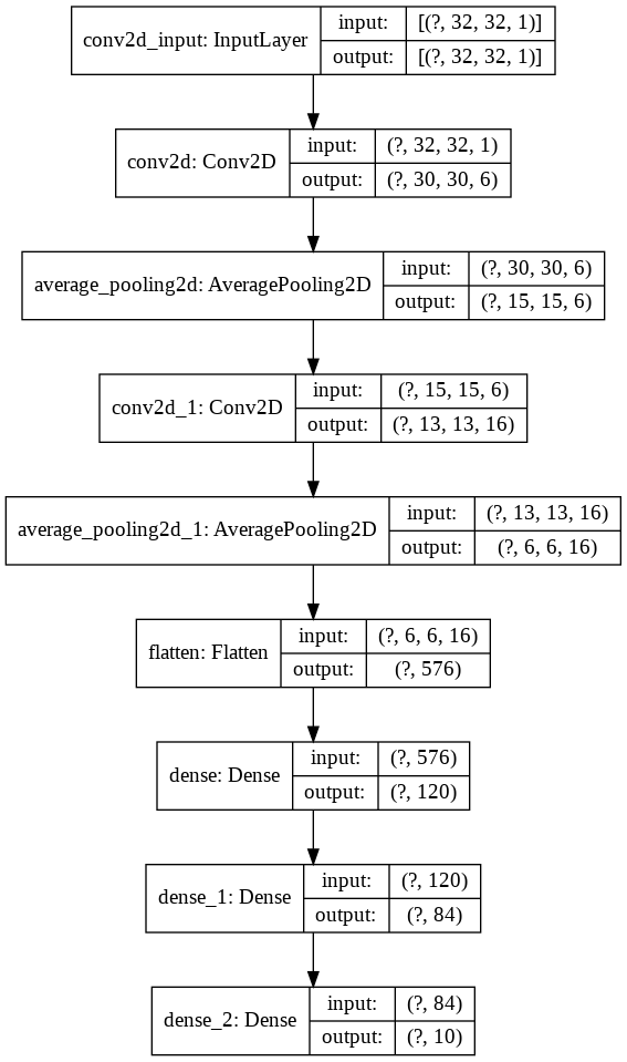
 import keras
from keras import layers
model = keras . Sequential ()

model . add ( layers . Conv2D ( filters = 6 , kernel_size = ( 3 , 3 ), activation = 'relu' , input_shape = ( 32 , 32 , 1 )))
model . add ( layers . AveragePooling2D ())

model . add ( layers . Conv2D ( filters = 16 , kernel_size = ( 3 , 3 ), activation = 'relu' ))
model . add ( layers . AveragePooling2D ())

model . add ( layers . Flatten ())

model . add ( layers . Dense ( units = 120 , activation = 'relu' ))

model . add ( layers . Dense ( units = 84 , activation = 'relu' ))

model . add ( layers . Dense ( units = 10 , activation = 'softmax' ))
Lassen Sie uns dies nun visualisieren
nn_visualize ( model )Standardmäßig gibt es ein Keras -Visualisierungsobjekt zurück
 from keras . models import Sequential
from keras . layers import Dense
import numpy
# fix random seed for reproducibility
numpy . random . seed ( 7 )
# load pima indians dataset
dataset = numpy . loadtxt ( "pima-indians-diabetes.csv" , delimiter = "," )
# split into input (X) and output (Y) variables
X = dataset [:, 0 : 8 ]
Y = dataset [:, 8 ]
# create model
model = Sequential ()
model . add ( Dense ( 12 , input_dim = 8 , activation = 'relu' ))
model . add ( Dense ( 8 , activation = 'relu' ))
model . add ( Dense ( 1 , activation = 'sigmoid' ))
# Compile model
model . compile ( loss = 'binary_crossentropy' , optimizer = 'adam' , metrics = [ 'accuracy' ])
# Fit the model
model . fit ( X , Y , epochs = 150 , batch_size = 10 )
# evaluate the model
scores = model . evaluate ( X , Y )
print ( " n %s: %.2f%%" % ( model . metrics_names [ 1 ], scores [ 1 ] * 100 ))


#Neural network visualization

nn_visualize ( model , type = "graphviz" )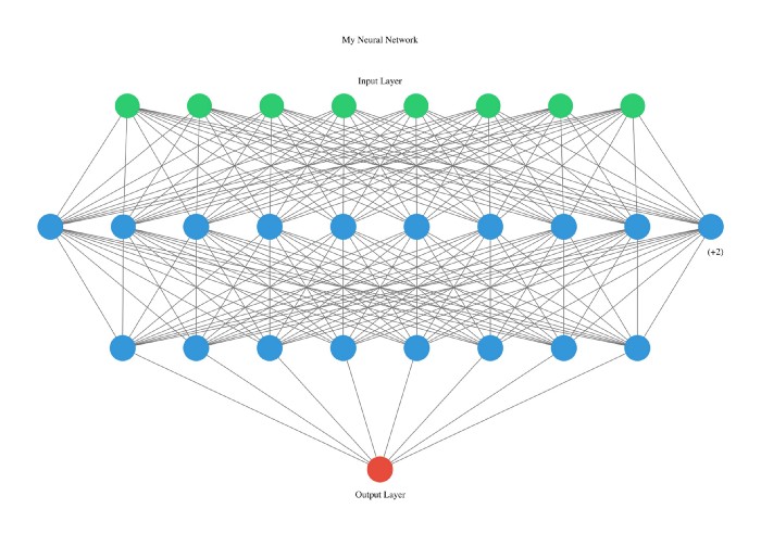
Diese Bibliothek ist so Entwickler freundlich, dass sogar wir den Typ mit Startbriefen deklarieren.
 from pyAutoML . model import *
model2 = model ( arch = "alexNet" )

nn_visualize ( model2 , type = "k" )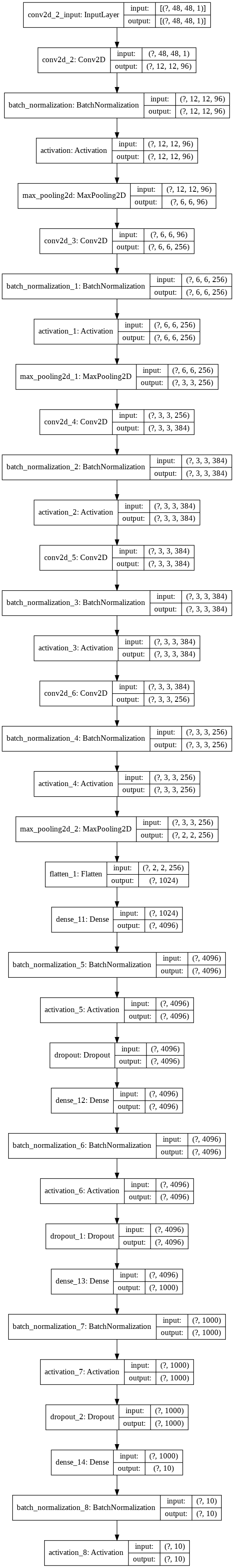
LinkedIn
Github
Instagram


