PhysicsExp
1.0.0
The package is also released on pypi.
For readers from pypi, here please.
For my experimental data and data processing scripts, pictures, and calculation results (from level 1 to level 4), please refer to the USTCPhysExpData project. My experiment data, data processing scripts, figures, and some results(from experiment level I to IV), please visit the USTCPhysExpData project.
Don't want to use OriginLab or Excel? Try Python!
The ultimate goal is to build a set of tools for automatically processing large object experimental data, drawing images, generating printable documents, and submitting documents to online printing systems; simplifying and automation is achieved for common data processing needs. With just a few simple lines of code, common tasks such as large object experiments such as drawing, fitting, uncertainty calculation can be completed.
There is still a big gap between ideal and reality. At present, only matplotlib drawing library, simple fitting, file input, and docx generation are packaged to simplify repetitive labor.
Now I only wrapped matplotlib plotting library, implemented simple regression, easy file input, and docx generation. To simplify repetious works.
Related blog: Pages on USTC LUG Pages on my homepage
Install the package
Use TUNA mirror to accelerate. Depenceencies like numpy and matplotlib will be installed automatically.
pip install -i https://mirrors.tuna.tsinghua.edu.cn/pypi/web/simple physicsexp
Test the installation(Optional)
 >>> from physicsexp.mainfunc import *
>>> from physicsexp.gendocx import *
>>>
If no error then you are ready! If error occurs feel free to open an issue.
Run the example script(Recommended)
python3 ./physicsexp/example/plot.py
You'll see graphs popped out and saved to .png, a generated gen.docx ready to print, and calculations printed to output, in the ./physicsexp/example directory. You can also clone USTCPhysExpData to try some real-life cases. Then you can modify the code or write your own code to process your data!
It is a real-case example of input several lines of data, plot the data and do linear regression, and generate a printable docx document containing plot and analyze results.
If you really want to know, the experiment is about verifying the relative kinetic energy vs. momentum relationship of electron(beta-ray) and measuring the extraction of beta-ray by aluminum pieces of different thickness.
First, put your data in data.txt , like this:
 # 位置x
e -2
23.     24.2    25.5    26.5    27.7    29.     30.5    31.8
# 峰位N
245.77  291.79  336.40  378.52  417.94  456.14  510.12  544.95
# 铝片数量M
0       1       2       3       4       5
# 选区计数N
43901   34258   28725   23670   19386   16866
You can use # to add some comment lines, and e * to specify the order of magnitude -- thus be able to directly write down the original on-paper data without conversion.
Then it's time to write python
Headers & imports
 #!/usr/bin/env python3
# -*- coding: utf-8 -*-

from physicsexp . mainfunc import *
from physicsexp . gendocx import *
Read the file easily with the readoneline function
 fin = open ( './data.txt' , 'r' , encoding = 'utf-8' )
pos = readoneline ( fin )
N = readoneline ( fin )
Al_num = readoneline ( fin )
Cnt = readoneline ( fin )
fin . close ()
Calculate and print some results. This is python, you can do whatever you like easily. (This part is not related to the library, you can skip this)
 a = 2.373e-3
b = - .0161
dEk = .20

c0 = 299792458.
MeV = 1e6 * electron

Emeasure = a * N + b + dEk
x0 = .10
R = ( pos - x0 ) / 2
B = 640.01e-4
Momentum = 300 * B * R
Eclassic = (( Momentum * MeV ) ** 2 / ( 2 * me * c0 ** 2 )) / MeV
Erela = np . array ([ math . sqrt (( i * MeV ) ** 2 + ( me * c0 ** 2 ) ** 2 ) - me * c0 ** 2 for i in Momentum ]) / MeV
print ( 'pos t ' , pos )
print ( 'R t ' , R * 100 )
print ( 'pc t ' , Momentum )
print ( 'N t ' , N )
print ( 'Eclas t ' , Eclassic )
print ( 'Erela t ' , Erela )
print ( 'Emes t ' , Emeasure )
Now, plot!
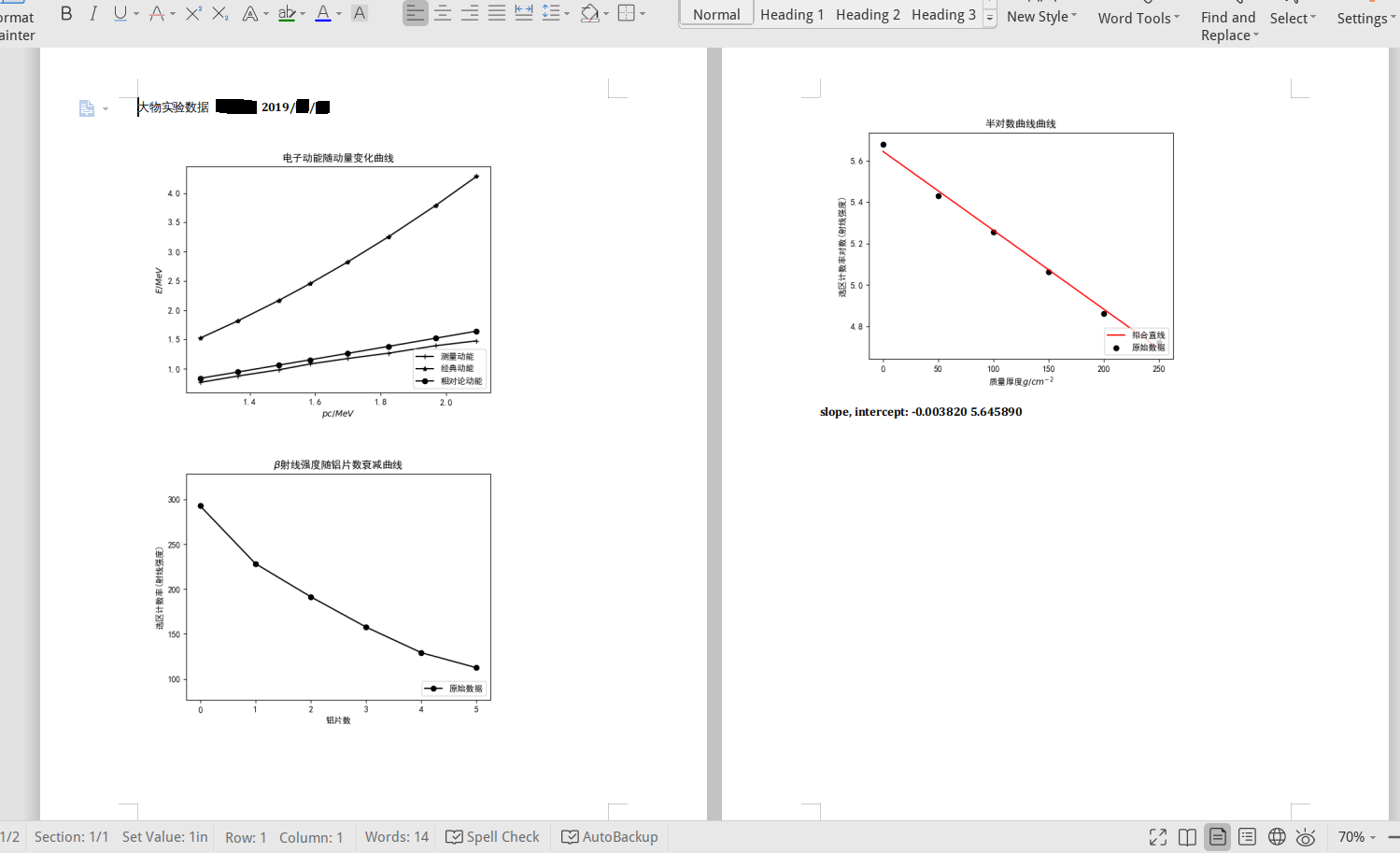
First graph: three curve in one figure. Using simple_plot . You can use LaTeX in plot labels. Graph is saved to 1.png . Use show=0 to plot multiple lines on one figure.
 simple_plot ( Momentum , Emeasure , show = 0 , issetrange = 0 , dot = '+' , lab = '测量动能' )
simple_plot ( Momentum , Eclassic , show = 0 , issetrange = 0 , dot = '*' , lab = '经典动能' )
simple_plot ( Momentum , Erela , dot = 'o' , save = '1.png' , issetrange = 0 , xlab = '$pc/MeV$' , ylab = '$E/MeV$' , title = '电子动能随动量变化曲线' , lab = '相对论动能' )
Second graph, a simple curve, saved to 2.png :
 Len = 150
Cnt = Cnt / Len
simple_plot ( Al_num , Cnt , xlab = '铝片数' , ylab = '选区计数率(射线强度)' , title = '$ \ beta$射线强度随铝片数衰减曲线' , save = '2.png' )
Third graph, a curve with a linear fit, using simple_linear_plot , saved to 3.png :
 CntLn = np . log ( Cnt )
d = 50
Al_Real = Al_num * d
slope , intercept = simple_linear_plot ( Al_Real , CntLn , xlab = '质量厚度$g/cm^{-2}$' , ylab = '选区计数率对数(射线强度)' , title = '半对数曲线曲线' , save = '3.png' )
print ( - slope )
print ( math . log ( 1e4 ) / ( - slope ))
print (( math . log ( Cnt [ 0 ]) - 4 * math . log ( 10 ) - intercept ) / slope )
Don't both putting pictures in documents yourself!
With a single line of code, generate a printable docx document with the above three pictures and the fit results.
gendocx ( 'gen.docx' , '1.png' , '2.png' , '3.png' , 'slope, intercept: %f %f' % ( slope , intercept ))Results
Output:
 pos	 [0.23  0.242 0.255 0.265 0.277 0.29  0.305 0.318]
R	 [ 6.5   7.1   7.75  8.25  8.85  9.5  10.25 10.9 ]
pc	 [1.2480195  1.3632213  1.48802325 1.58402475 1.69922655 1.8240285
 1.96803075 2.0928327 ]
N	 [245.77 291.79 336.4  378.52 417.94 456.14 510.12 544.95]
Eclas	 [1.52375616 1.81804848 2.16616816 2.45469003 2.82471934 3.25488743
 3.78910372 4.28491053]
Erela	 [0.83752628 0.94478965 1.0622588  1.15334615 1.26333503 1.3831891
 1.52222218 1.64324566]
Emes	 [0.76711221 0.87631767 0.9821772  1.08212796 1.17567162 1.26632022
 1.39441476 1.47706635]
0.0038199159787357996
2411.136900195471
2402.45428200782
Generated docx:
Don't forget to change my name to yours.
Later I found that using jupyter notebook is WAY MUCH better than coding in python editor:
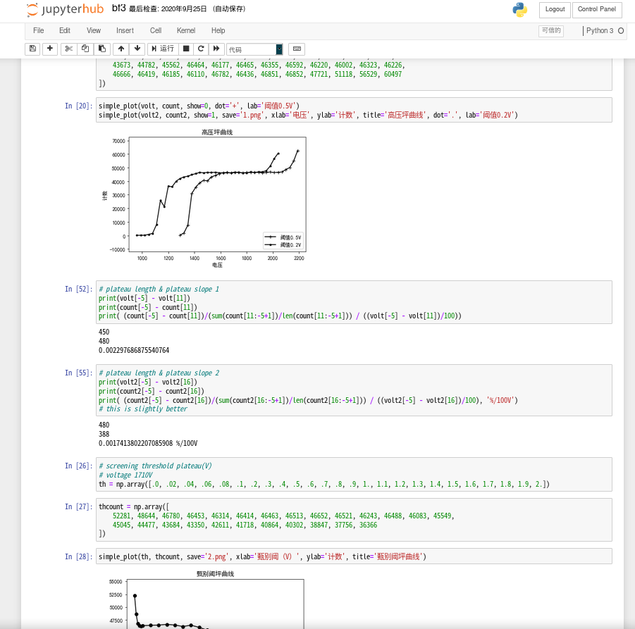
And, Jupyterhub can provide jupyter notebook access for a group of users: the common case when several people want to share their experiment data processing script with each other.
In ./jupyterhub is my config being used to run jupyterhub: docker spawner with a shared struggle, dummy authentication. Literally no security or access control but acceptable for a group of trustable people on a private server.
Wanna know how to use after reading the example?
You can:
However, they are not intended to run directly on your machine and magically give you correct answer without any change, but, if you really want to run them, maybe a
git reseton this repository and dive into the dark history is the last resort.
Read the source code yourself. Especially physicsexp/mainfunc.py and physicsexp/gendocx.py -- with the example covering most use cases, you just need to check out function declaration and extra available options(they make life easier).
Or open an issue. If you are also a USTC student just contact me with QQ/Email. Contacts are on my website.
But don't be frustrated if none of these works. The project comes with absolutely no warning.
And can using these tools boost your efficiency? I don't know, but probably can't.
**However, if these can make you feel better despite spending more time, use it. **
Finally, think twice before wasting time on this project, instead, enjoy your life, learn some real physics, and find a (boy|girl)friend.
Here.


