cufflinks
1.0.0
Diese Bibliothek bindet die Leistung von Plotly mit der Flexibilität von Pandas für das einfache Planen.
Diese Bibliothek ist unter https://github.com/santosjorge/cufflinks verfügbar
In diesem Tutorial geht davon aus, dass die Plotly -Benutzer -Anmeldeinformationen bereits wie im Handbuch für Erste Schritte angegeben wurden.
Unterstützung für Plotly 4.x
Manschettenknöpfe sind nicht mehr mit Plotly 3.x kompatibel
Unterstützung für Plotly 3.0
NEU iplot HELPER. Um eine umfassende Liste von Parametern zu sehen , vgl. Help ()
 # For a list of supported figures
cf . help ()
# Or to see the parameters supported that apply to a given figure try
cf . help ( 'scatter' )
cf . help ( 'candle' ) #etcAbhängige auf Ta-Lib entfernt. Diese Bibliothek ist nicht mehr erforderlich. Alle Studien wurden in Python umgeschrieben.
QuantFigure ist eine neue Klasse, die ein Diagrammobjekt mit Persistenz erzeugt. Parameter können an einem bestimmten Punkt hinzugefügt/geändert werden.Dies kann so einfach sein wie:
 df = cf . datagen . ohlc ()
qf = cf . QuantFig ( df , title = 'First Quant Figure' , legend = 'top' , name = 'GS' )
qf . add_bollinger_bands ()
qf . iplot ()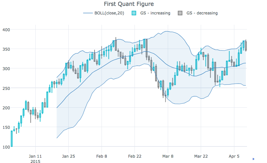
 qf . add_sma ([ 10 , 20 ], width = 2 , color = [ 'green' , 'lightgreen' ], legendgroup = True )
qf . add_rsi ( periods = 20 , color = 'java' )
qf . add_bollinger_bands ( periods = 20 , boll_std = 2 , colors = [ 'magenta' , 'grey' ], fill = True )
qf . add_volume ()
qf . add_macd ()
qf . iplot ()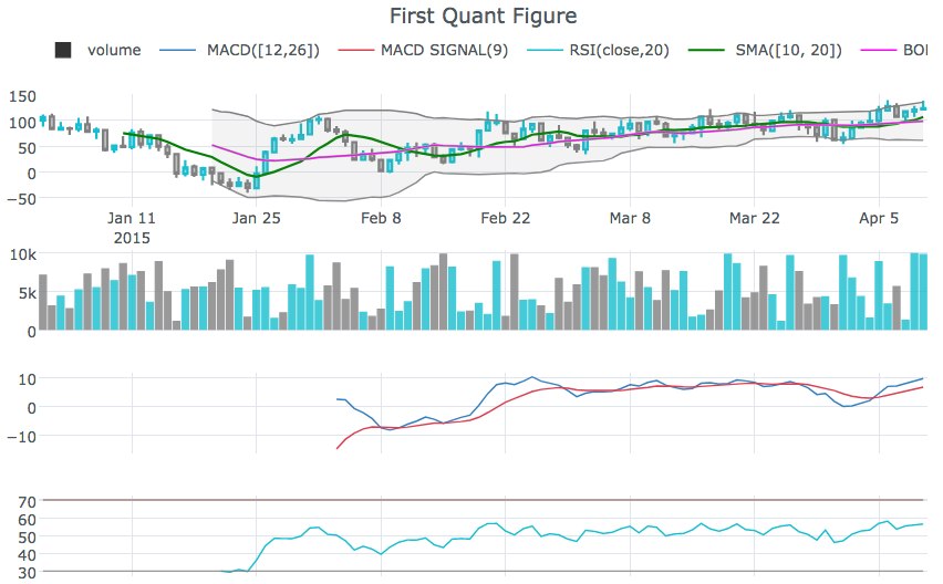
rangeslider um einen Date -Bereichs -Schieberegler unten anzuzeigencf.datagen.ohlc().iplot(kind='candle',rangeslider=True)rangeselector um Schaltflächen anzuzeigen, um den angezeigten Datumsbereich zu änderncf.datagen.ohlc(500).iplot(kind='candle', rangeselector={ 'steps':['1y','2 months','5 weeks','ytd','2mtd','reset'], 'bgcolor' : ('grey',.3), 'x': 0.3 , 'y' : 0.95})fontsize , fontcolor , textanglecf.datagen.lines(1,mode='stocks').iplot(kind='line', annotations={'2015-02-02':'Market Crash', '2015-03-01':'Recovery'}, textangle=-70,fontsize=13,fontcolor='grey')cf.datagen.lines(1,mode='stocks').iplot(kind='line', annotations=[{'text':'exactly here','x':'0.2', 'xref':'paper','arrowhead':2, 'textangle':-10,'ay':150,'arrowcolor':'red'}])Figure.iplot() um Abbildungen zu zeichnencf.datagen.ohlc().iplot(kind='candle')iplotxrange , yrange und zrange können in iplot und getLayout angegeben werdencf.datagen.lines(1).iplot(yrange=[5,15])layout_update kann in iplot eingestellt werden und getLayout Layout explizit aktualisierenSiehe das Ipython -Notizbuch
cf.datagen.pie().iplot(kind='pie',labels='labels',values='values')datagen.ohlc()ohlc=cf.datagen.ohlc()ohlc.iplot(kind='candle',up_color='blue',down_color='red')ohlc=cf.datagen.ohlc()ohlc.iplot(kind='ohlc',up_color='blue',down_color='red')df=pd.DataFrame([x**2] for x in range(100))df.iplot(kind='lines',logy=True)cf.datagen.lines(1,5).iplot(kind='bar',error_y=[1,2,3.5,2,2])cf.datagen.lines(1,5).iplot(kind='bar',error_y=20, error_type='percent')cf.datagen.lines(1).iplot(kind='lines',error_y=20,error_type='continuous_percent')cf.datagen.lines(1).iplot(kind='lines',error_y=10,error_type='continuous',color='blue')cf.datagen.lines(1,500).ta_plot(study='sma',periods=[13,21,55])cf.datagen.lines(1,200).ta_plot(study='boll',periods=14)cf.datagen.lines(1,200).ta_plot(study='rsi',periods=14)cf.datagen.lines(1,200).ta_plot(study='macd',fast_period=12,slow_period=26, signal_period=9)cf.go_offline()cf.go_online()cf.iplot(figure,online=True) (online im Offline -Modus zu erzwingen)fig=cf.datagen.lines(3,columns=['a','b','c']).figure()fig=fig.set_axis('b',side='right')cf.iplot(fig)cufflinks.set_config_file(theme='pearl')cufflinks.datagen.lines(5).iplot(theme='ggplot')cufflinks.datagen.lines(2).iplot(kind='barh',barmode='stack',bargap=.1)cufflinks.datagen.histogram().iplot(kind='histogram',orientation='h',norm='probability')cufflinks.datagen.lines(4).iplot(kind='area',fill=True,opacity=1)cufflinks.datagen.histogram(4).iplot(kind='histogram',subplots=True,bins=50)cufflinks.datagen.lines(4).iplot(subplots=True,shape=(4,1),shared_xaxes=True,vertical_spacing=.02,fill=True)cufflinks.datagen.lines(4,1000).scatter_matrix()cufflinks.datagen.lines(3).iplot(hline=[2,3])cufflinks.datagen.lines(3).iplot(hline=dict(y=2,color='blue',width=3))cufflinks.datagen.lines(3).iplot(hspan=(-1,2))cufflinks.datagen.lines(3).iplot(hspan=dict(y0=-1,y1=2,color='orange',fill=True,opacity=.4))cufflinks.set_config_file(world_readable=True)cufflinks.datagen.lines(2).iplot(kind='spread')cufflinks.datagen.heatmap().iplot(kind='heatmap')cufflinks.datagen.bubble(4).iplot(kind='bubble',x='x',y='y',text='text',size='size',categories='categories')cufflinks.datagen.bubble3d(4).iplot(kind='bubble3d',x='x',y='y',z='z',text='text',size='size',categories='categories')cufflinks.datagen.box().iplot(kind='box')cufflinks.datagen.surface().iplot(kind='surface')cufflinks.datagen.scatter3d().iplot(kind='scatter3d',x='x',y='y',z='z',text='text',categories='categories')cufflinks.datagen.histogram(2).iplot(kind='histogram')cufflinks.datagencufflinks.to_df(Figure)iplot(colorscale='accent') um ein Diagramm mit einer Akzentfarbe zu zeichneniplot(colors=['pink','red','yellow'])

