OpenAI CLIP
openai-clip-first-release
我很高興發現該代碼已在以下論文中使用和引用:
多米諾骨牌: Eyuboglu et Life-toss-Modal嵌入的系統誤差。 al。在ICLR 2022
GSCLIP: Zhu等人解釋自然語言分佈變化的框架。 al。在ICML 2022
semeval-2022任務5:探索Cuervo等人對厭惡女性模因的多模式檢測的對比學習。 al。在Semeval-2022
CDSBERT- HALLEE等人的密碼子意識擴展蛋白質語言模型。 al。來自特拉華大學(2023年9月)
Enigma-51:在Ragusa等人的工業場景中對人類對象的相互作用進行細粒度的了解。 al。 (2023年11月)
您可以在此GitHub存儲庫頁面的正確部分上找到命名的引用信息:引用此存儲庫或使用以下引用信息。
 @software { Shariatnia_Simple_CLIP_2021 ,
author = { Shariatnia, M. Moein } ,
doi = { 10.5281/zenodo.6845731 } ,
month = { 4 } ,
title = { {Simple CLIP} } ,
version = { 1.0.0 } ,
year = { 2021 }
}在2021年1月, Openai宣布了兩個新型號: Dall-E和Clip ,這兩種模型都以某種方式連接文本和圖像。在本文中,我們將在Pytorch中從頭開始實現剪輯模型。 Openai開源了一些與剪輯模型有關的代碼,但我發現它令人生畏,而且遠非簡短而簡單。我還遇到了一個很好的教程,該教程靈感來自Keras Code示例的剪輯模型,然後將其中的某些部分翻譯成Pytorch,以完全使用我們心愛的Pytorch構建本教程!
在從自然語言監督論文中學習可轉移的視覺模型時,OpenAI介紹了其新模型,該模型稱為剪輯,以進行對比語言圖像預訓練。簡而言之,該模型了解了整個句子與其描述的圖像之間的關係。從某種意義上說,當訓練模型時,鑑於輸入句子,它將能夠檢索與該句子相對應的最相關的圖像。這裡重要的是,它是對完整句子的培訓,而不是諸如汽車,狗等的單一類培訓。直覺是,在對整個句子進行培訓時,該模型可以學習更多的東西,並在圖像和文本之間找到一些模式。他們還表明,當該模型在龐大的圖像數據集及其相應的文本中訓練時,它也可以充當分類器。我鼓勵您研究論文,以了解有關這種令人興奮的模型及其在基準數據集中的驚人結果的更多信息。僅提到,使用此策略訓練的剪輯模型比在ImageNet本身中針對唯一的分類任務進行了優化的SOTA模型,對IMATENET進行了訓練!
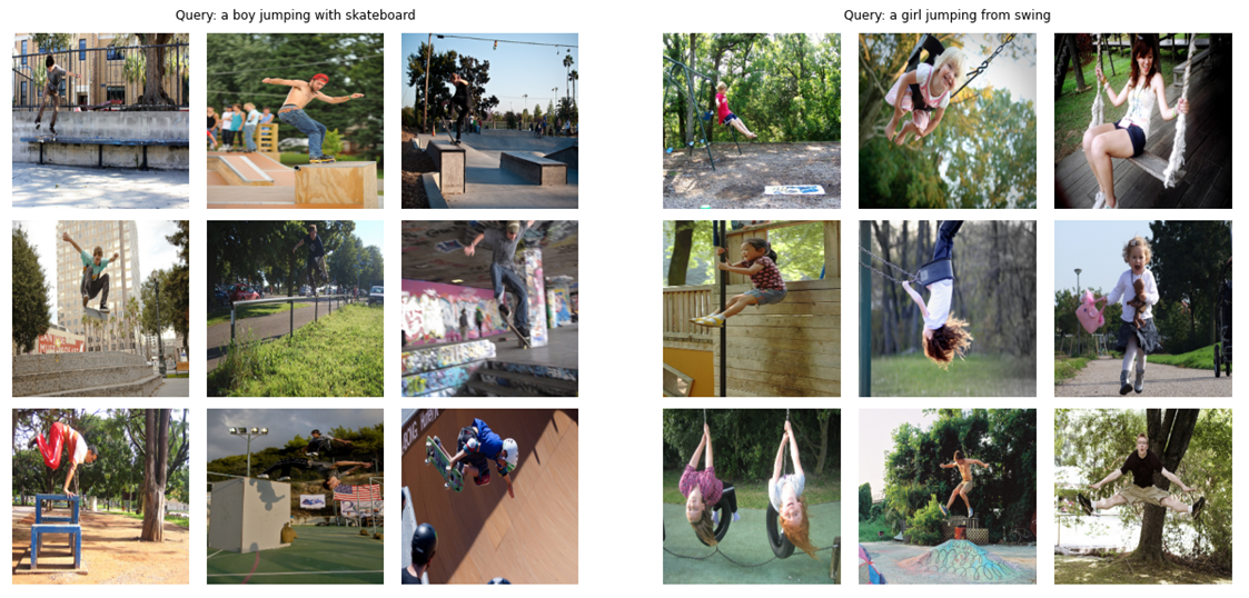
作為一個預告片(!),讓我們看看我們將在本文中從頭開始構建的最終模型能夠:給定查詢(原始文本),例如“一個男孩跳滑板跳著滑板”或“從鞦韆上跳下來的女孩”,該模型將檢索最相關的圖像:
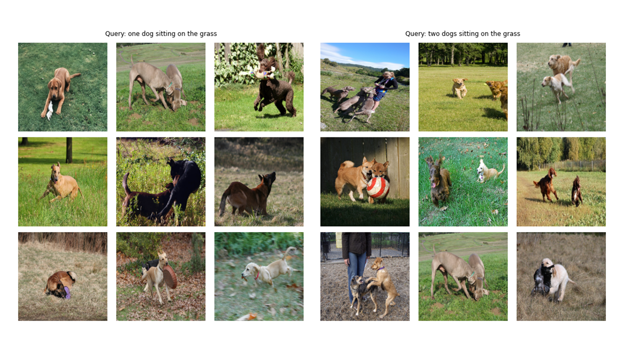
讓我們看看更多的輸出:
 # !pip install timm
# !pip install transformers
import os
import cv2
import gc
import numpy as np
import pandas as pd
import itertools
from tqdm . autonotebook import tqdm
import albumentations as A
import torch
from torch import nn
import torch . nn . functional as F
import timm
from transformers import DistilBertModel , DistilBertConfig , DistilBertTokenizer 關於Config和CFG的註釋:我用Python腳本編寫了代碼,然後將其轉換為Jupyter筆記本。因此,在Python腳本的情況下,配置是一個普通的Python文件,我將所有超參數放置在其中,而對於Jupyter Notebook,它是在筆記本開始時定義的類,以保留所有超級參數。
 class CFG :
    debug = False
    image_path = "C:/Moein/AI/Datasets/Flicker-8k/Images"
    captions_path = "C:/Moein/AI/Datasets/Flicker-8k"
    batch_size = 32
    num_workers = 4
    head_lr = 1e-3
    image_encoder_lr = 1e-4
    text_encoder_lr = 1e-5
    weight_decay = 1e-3
    patience = 1
    factor = 0.8
    epochs = 4
    device = torch . device ( "cuda" if torch . cuda . is_available () else "cpu" )

    model_name = 'resnet50'
    image_embedding = 2048
    text_encoder_model = "distilbert-base-uncased"
    text_embedding = 768
    text_tokenizer = "distilbert-base-uncased"
    max_length = 200

    pretrained = True # for both image encoder and text encoder
    trainable = True # for both image encoder and text encoder
    temperature = 1.0

    # image size
    size = 224

    # for projection head; used for both image and text encoders
    num_projection_layers = 1
    projection_dim = 256
dropout = 0.1 class AvgMeter :
def __init__ ( self , name = "Metric" ):
self . name = name
self . reset ()
def reset ( self ):
self . avg , self . sum , self . count = [ 0 ] * 3
def update ( self , val , count = 1 ):
self . count += count
self . sum += val * count
self . avg = self . sum / self . count
def __repr__ ( self ):
text = f" { self . name } : { self . avg :.4f } "
return text
def get_lr ( optimizer ):
for param_group in optimizer . param_groups :
return param_group [ "lr" ]正如您在本文的圖像中看到的那樣,我們需要對圖像及其描述文本進行編碼。因此,數據集需要返回圖像和文本。當然,我們不會將原始文本饋送到我們的文本編碼器!我們將使用HuggingFace庫中的Distilbert模型(比Bert小,但表現差不多)與我們的文本編碼器一樣;因此,我們需要用Diskilbert Tokenizer將句子(字幕)歸為句子(字幕),然後將令牌ID(Input_IDS)和注意力掩蓋餵入Distilbert。因此,數據集也需要照顧令牌化。在下面,您可以看到數據集的代碼。在此下面,我將解釋代碼中最重要的事情。
在__init__中,我們會收到一個令牌對象,這實際上是一個擁抱面托犬。運行模型時將加載此令牌。我們正在將字幕填充並截斷為指定的max_length。在__getItem__中,我們將首先加載一個編碼的標題,該字典是帶有鍵input_ids和coative_mask的字典,使張量從其值中取出,然後我們將加載相應的映像,轉換和增強它(如果有任何!最後,我們僅出於可視化目的將標題的原始文本放入字典中的鍵“標題”。
我沒有使用其他數據增強,但是如果您想提高模型的性能,則可以添加它們。
 class CLIPDataset ( torch . utils . data . Dataset ):
    def __init__ ( self , image_filenames , captions , tokenizer , transforms ):
        """
        image_filenames and cpations must have the same length; so, if there are
        multiple captions for each image, the image_filenames must have repetitive
        file names
        """

        self . image_filenames = image_filenames
        self . captions = list ( captions )
        self . encoded_captions = tokenizer (
            list ( captions ), padding = True , truncation = True , max_length = CFG . max_length
        )
        self . transforms = transforms

    def __getitem__ ( self , idx ):
        item = {
            key : torch . tensor ( values [ idx ])
            for key , values in self . encoded_captions . items ()
        }

        image = cv2 . imread ( f" { CFG . image_path } / { self . image_filenames [ idx ] } " )
        image = cv2 . cvtColor ( image , cv2 . COLOR_BGR2RGB )
        image = self . transforms ( image = image )[ 'image' ]
        item [ 'image' ] = torch . tensor ( image ). permute ( 2 , 0 , 1 ). float ()
        item [ 'caption' ] = self . captions [ idx ]

        return item


    def __len__ ( self ):
        return len ( self . captions )


def get_transforms ( mode = "train" ):
    if mode == "train" :
        return A . Compose (
            [
                A . Resize ( CFG . size , CFG . size , always_apply = True ),
                A . Normalize ( max_pixel_value = 255.0 , always_apply = True ),
            ]
        )
    else :
        return A . Compose (
            [
                A . Resize ( CFG . size , CFG . size , always_apply = True ),
                A . Normalize ( max_pixel_value = 255.0 , always_apply = True ),
            ]
)圖像編碼器代碼直截了當。我在此處使用Pytorch Image Models庫(TIMM),這使許多不同的映像模型可從Resnets到EditiveNets等等。在這裡,我們將使用Resnet50作為圖像編碼器。如果您不想安裝新庫,則可以輕鬆使用Torchvision庫使用Resnets。
代碼將每個圖像編碼為固定大小向量,並具有模型輸出通道的大小(如果是Resnet50,則向量大小為2048 )。這是NN.Adaptiveavgpool2d()層之後的輸出。
 class ImageEncoder ( nn . Module ):
    """
    Encode images to a fixed size vector
    """

    def __init__ (
        self , model_name = CFG . model_name , pretrained = CFG . pretrained , trainable = CFG . trainable
    ):
        super (). __init__ ()
        self . model = timm . create_model (
            model_name , pretrained , num_classes = 0 , global_pool = "avg"
        )
        for p in self . model . parameters ():
            p . requires_grad = trainable

    def forward ( self , x ):
return self . model ( x )正如我之前提到的,我將使用Distilbert作為文本編碼器。像更大的兄弟伯特一樣,將添加兩個特殊的令牌: CLS和SEP的實際輸入令牌:標誌著句子的開始和結尾。為了抓住句子的全部表示(如相關的Bert和Distilbert Papers所指出的那樣),我們使用CLS令牌的最終表示形式,我們希望這種表示能夠捕獲句子的整體含義(標題)。以這種方式思考,它類似於我們對圖像所做的事情,並將它們轉換為固定尺寸的向量。
在Distilbert(以及Bert)的情況下,每個令牌的輸出隱藏表示形式是一個尺寸768的向量。因此,整個標題將在大小為768的CLS令牌表示中編碼。
 class TextEncoder ( nn . Module ):
    def __init__ ( self , model_name = CFG . text_encoder_model , pretrained = CFG . pretrained , trainable = CFG . trainable ):
        super (). __init__ ()
        if pretrained :
            self . model = DistilBertModel . from_pretrained ( model_name )
        else :
            self . model = DistilBertModel ( config = DistilBertConfig ())

        for p in self . model . parameters ():
            p . requires_grad = trainable

        # we are using the CLS token hidden representation as the sentence's embedding
        self . target_token_idx = 0

    def forward ( self , input_ids , attention_mask ):
        output = self . model ( input_ids = input_ids , attention_mask = attention_mask )
        last_hidden_state = output . last_hidden_state
return last_hidden_state [:, self . target_token_idx , :]我使用KERAS代碼示例的投影頭實現來在Pytorch中編寫以下內容。現在,我們已經將圖像和文本編碼為固定尺寸的向量(圖像為2048,文本為768),我們需要將它們(項目)帶入一個新世界(!),圖像和文本都具有相似的尺寸,以便能夠比較它們並將其推開,並將其推開,並將其推開,並將非相關的圖像和文本與匹配的那些匹配的圖像和文本拉在一起。因此,以下代碼將使2048和768維向量進入256(投射_dim)維度世界,我們可以在其中比較它們。
“ embedding_dim”是輸入向量的大小(圖像的2048,文本為768)和“ propption_dim”是輸出向量的大小,我們的情況將為256。為了了解此部分的詳細信息,您可以參考剪輯紙。
 class ProjectionHead ( nn . Module ):
    def __init__ (
        self ,
        embedding_dim ,
        projection_dim = CFG . projection_dim ,
        dropout = CFG . dropout
    ):
        super (). __init__ ()
        self . projection = nn . Linear ( embedding_dim , projection_dim )
        self . gelu = nn . GELU ()
        self . fc = nn . Linear ( projection_dim , projection_dim )
        self . dropout = nn . Dropout ( dropout )
        self . layer_norm = nn . LayerNorm ( projection_dim )

    def forward ( self , x ):
        projected = self . projection ( x )
        x = self . gelu ( projected )
        x = self . fc ( x )
        x = self . dropout ( x )
        x = x + projected
        x = self . layer_norm ( x )
return x 這部分是所有樂趣發生的地方!我還將在這裡談論損失功能。我將一些代碼從KERAS代碼示例轉換為Pytorch,以編寫此部分。查看代碼,然後閱讀此代碼塊下面的說明。
在這裡,我們將使用我們構建的先前模塊來實現主模型。 __init__函數是自我解釋的。在正向函數中,我們首先將圖像和文本分別編碼為固定尺寸向量(具有不同的維度)。之後,使用單獨的投影模塊,我們將它們投影到我之前談到的那個共享世界(空間)。在這裡,編碼將變成相似的形狀(在我們的情況下為256)。之後,我們將計算損失。再次,我建議閱讀剪貼紙以使其變得更好,但我會盡力解釋這部分。
在線性代數中,測量兩個向量是否具有相似特徵(它們彼此相似)的一種常見方法是計算其點產物(乘以匹配的條目並拿走它們的總和);如果最終數量很大,那麼它們是相同的,如果它很小,則不會(相對而言)!
好的!我剛才說的是要了解這種損失功能的最重要的事情。讓我們繼續。我們談到了兩個向量,但是,我們在這裡有什麼?我們有image_embeddings,具有形狀(batch_size,256)的矩陣和帶狀的text_embeddings(batch_size,256)。很容易!這意味著我們有兩組向量,而不是兩個向量。我們如何衡量類似的兩組向量(兩個矩陣)彼此之間的樣子?同樣,使用點產品(在這種情況下,Pytorch中的@運算符會執行點產品或矩陣乘法)。為了能夠將這兩個矩陣倍增,我們將第二個矩陣轉換。好的,我們獲得了一個帶有形狀的矩陣(batch_size,batch_size),我們將調用logits。 (在我們的情況下,溫度等於1.0,因此,它不會有所作為。您可以使用它並查看它的差異。還請查看紙張以查看為什麼它在這裡!)。
我希望你仍然和我在一起!如果沒有,請檢查代碼並檢查其形狀。現在我們有了邏輯,我們需要目標。我需要說,有一種更直接的方法來獲得目標,但我必須為我們的情況做到這一點(我將在下一段中談論為什麼)。
讓我們考慮一下我們希望該模型學習的內容:我們希望它為給定的圖像學習“相似的表示(向量)”和描述它的標題。這意味著我們要么給它一個圖像,要么是描述它的文本,我們希望它為兩者產生相同的256個大小的向量。
 class CLIPModel ( nn . Module ):
    def __init__ (
        self ,
        temperature = CFG . temperature ,
        image_embedding = CFG . image_embedding ,
        text_embedding = CFG . text_embedding ,
    ):
        super (). __init__ ()
        self . image_encoder = ImageEncoder ()
        self . text_encoder = TextEncoder ()
        self . image_projection = ProjectionHead ( embedding_dim = image_embedding )
        self . text_projection = ProjectionHead ( embedding_dim = text_embedding )
        self . temperature = temperature

    def forward ( self , batch ):
        # Getting Image and Text Features
        image_features = self . image_encoder ( batch [ "image" ])
        text_features = self . text_encoder (
            input_ids = batch [ "input_ids" ], attention_mask = batch [ "attention_mask" ]
        )
        # Getting Image and Text Embeddings (with same dimension)
        image_embeddings = self . image_projection ( image_features )
        text_embeddings = self . text_projection ( text_features )

        # Calculating the Loss
        logits = ( text_embeddings @ image_embeddings . T ) / self . temperature
        images_similarity = image_embeddings @ image_embeddings . T
        texts_similarity = text_embeddings @ text_embeddings . T
        targets = F . softmax (
            ( images_similarity + texts_similarity ) / 2 * self . temperature , dim = - 1
        )
        texts_loss = cross_entropy ( logits , targets , reduction = 'none' )
        images_loss = cross_entropy ( logits . T , targets . T , reduction = 'none' )
        loss =  ( images_loss + texts_loss ) / 2.0 # shape: (batch_size)
        return loss . mean ()


def cross_entropy ( preds , targets , reduction = 'none' ):
    log_softmax = nn . LogSoftmax ( dim = - 1 )
    loss = ( - targets * log_softmax ( preds )). sum ( 1 )
    if reduction == "none" :
        return loss
    elif reduction == "mean" :
        return loss . mean ()
因此,在最佳情況下,text_embeddings和image_embedding矩陣應該相同,因為它們正在描述類似的內容。現在讓我們考慮一下:如果發生這種情況,logits矩陣會是什麼樣?讓我們看看一個簡單的例子!
 # A simple Example

batch_size = 4
dim = 256
embeddings = torch . randn ( batch_size , dim )
out = embeddings @ embeddings . T
print ( F . softmax ( out , dim = - 1 ))
因此,在最好的情況下,logits將是一個矩陣,如果我們採用其SoftMax,在對角線中將具有1.0級(一個以精美的單詞來稱呼它的身份矩陣!)。由於損失函數的工作是使模型的預測與目標相似(至少在大多數情況下!),我們希望這樣的矩陣作為目標。這就是為什麼我們在上面的代碼塊中計算images_simurility和texts_simarlity矩陣的原因。
現在,我們已經擁有目標矩陣,我們將使用簡單的橫熵來計算實際損失。我已經將跨熵的完整矩陣形式寫為一個函數,您可以在代碼塊的底部看到。好的!我們完成了!這不是簡單嗎?好吧,您可以忽略下一個段落,但是如果您很好奇,那麼其中有一個重要的註釋。
這就是為什麼我沒有使用更簡單的方法:我需要承認有一種更簡單的方法來計算Pytorch中的這種損失;通過這樣做:nn.crossentropyloss()(logits,torch.arange(batch_size))。為什麼我在這裡不使用它?出於兩個原因。 1-我們正在使用的數據集具有單個圖像的多個字幕;因此,有可能在批處理中存在兩個具有相似標題的相同標題的相同圖像(很少見,但可能發生)。用這種更輕鬆的方法損失將忽略這種可能性,並且該模型學會了將兩個實際上相同的表示形式拉開(假設它們不同)。顯然,我們不希望發生這種情況,因此我以照顧這些邊緣情況的方式計算了整個目標矩陣。 2-按照我的方式這樣做,使我更好地了解了此損失功能中正在發生的事情;因此,我認為這也可以為您提供更好的直覺!
以下是一些功能,可以幫助我們加載火車和有效的數據加載器,我們的模型,然後訓練和評估我們的模型。這裡沒有太多發生。只是簡單的訓練循環和實用程序功能
 def make_train_valid_dfs ():
    dataframe = pd . read_csv ( f" { CFG . captions_path } /captions.csv" )
    max_id = dataframe [ "id" ]. max () + 1 if not CFG . debug else 100
    image_ids = np . arange ( 0 , max_id )
    np . random . seed ( 42 )
    valid_ids = np . random . choice (
        image_ids , size = int ( 0.2 * len ( image_ids )), replace = False
    )
    train_ids = [ id_ for id_ in image_ids if id_ not in valid_ids ]
    train_dataframe = dataframe [ dataframe [ "id" ]. isin ( train_ids )]. reset_index ( drop = True )
    valid_dataframe = dataframe [ dataframe [ "id" ]. isin ( valid_ids )]. reset_index ( drop = True )
    return train_dataframe , valid_dataframe


def build_loaders ( dataframe , tokenizer , mode ):
    transforms = get_transforms ( mode = mode )
    dataset = CLIPDataset (
        dataframe [ "image" ]. values ,
        dataframe [ "caption" ]. values ,
        tokenizer = tokenizer ,
        transforms = transforms ,
    )
    dataloader = torch . utils . data . DataLoader (
        dataset ,
        batch_size = CFG . batch_size ,
        num_workers = CFG . num_workers ,
        shuffle = True if mode == "train" else False ,
    )
    return dataloader
這是訓練我們的模型的方便功能。這裡沒有太多發生。只需加載批處理,將它們饋入模型,然後踩下優化器和LR_SCHEDULER。
 def train_epoch ( model , train_loader , optimizer , lr_scheduler , step ):
    loss_meter = AvgMeter ()
    tqdm_object = tqdm ( train_loader , total = len ( train_loader ))
    for batch in tqdm_object :
        batch = { k : v . to ( CFG . device ) for k , v in batch . items () if k != "caption" }
        loss = model ( batch )
        optimizer . zero_grad ()
        loss . backward ()
        optimizer . step ()
        if step == "batch" :
            lr_scheduler . step ()

        count = batch [ "image" ]. size ( 0 )
        loss_meter . update ( loss . item (), count )

        tqdm_object . set_postfix ( train_loss = loss_meter . avg , lr = get_lr ( optimizer ))
    return loss_meter


def valid_epoch ( model , valid_loader ):
    loss_meter = AvgMeter ()

    tqdm_object = tqdm ( valid_loader , total = len ( valid_loader ))
    for batch in tqdm_object :
        batch = { k : v . to ( CFG . device ) for k , v in batch . items () if k != "caption" }
        loss = model ( batch )

        count = batch [ "image" ]. size ( 0 )
        loss_meter . update ( loss . item (), count )

        tqdm_object . set_postfix ( valid_loss = loss_meter . avg )
    return loss_meter


def main ():
    train_df , valid_df = make_train_valid_dfs ()
    tokenizer = DistilBertTokenizer . from_pretrained ( CFG . text_tokenizer )
    train_loader = build_loaders ( train_df , tokenizer , mode = "train" )
    valid_loader = build_loaders ( valid_df , tokenizer , mode = "valid" )


    model = CLIPModel (). to ( CFG . device )
    params = [
        { "params" : model . image_encoder . parameters (), "lr" : CFG . image_encoder_lr },
        { "params" : model . text_encoder . parameters (), "lr" : CFG . text_encoder_lr },
        { "params" : itertools . chain (
            model . image_projection . parameters (), model . text_projection . parameters ()
        ), "lr" : CFG . head_lr , "weight_decay" : CFG . weight_decay }
    ]
    optimizer = torch . optim . AdamW ( params , weight_decay = 0. )
    lr_scheduler = torch . optim . lr_scheduler . ReduceLROnPlateau (
        optimizer , mode = "min" , patience = CFG . patience , factor = CFG . factor
    )
    step = "epoch"

    best_loss = float ( 'inf' )
    for epoch in range ( CFG . epochs ):
        print ( f"Epoch: { epoch + 1 } " )
        model . train ()
        train_loss = train_epoch ( model , train_loader , optimizer , lr_scheduler , step )
        model . eval ()
        with torch . no_grad ():
            valid_loss = valid_epoch ( model , valid_loader )

        if valid_loss . avg < best_loss :
            best_loss = valid_loss . avg
            torch . save ( model . state_dict (), "best.pt" )
            print ( "Saved Best Model!" )

        lr_scheduler . step ( valid_loss . avg )
運行下一個單元格啟動訓練模型。將內核處於GPU模式。每個時代都應在GPU上花費大約24分鐘(即使一個時代就足夠了!)。可能需要一分鐘的時間才能真正開始訓練,因為我們將在火車和有效數據集中編碼所有字幕,因此請不要停止它!每件事都很好。
main ()好的!我們已經完成了訓練模型。現在,我們需要進行推斷,在我們的情況下,這將為模型提供一條文本,並希望它從看不見的驗證(或測試)集中檢索最相關的圖像。
在此功能中,我們正在加載訓練後保存的模型,以驗證設置為IT圖像饋送圖像,並以Shape(valif_set_size,256)和模型本身返回image_embeddings。
 def get_image_embeddings ( valid_df , model_path ):
    tokenizer = DistilBertTokenizer . from_pretrained ( CFG . text_tokenizer )
    valid_loader = build_loaders ( valid_df , tokenizer , mode = "valid" )

    model = CLIPModel (). to ( CFG . device )
    model . load_state_dict ( torch . load ( model_path , map_location = CFG . device ))
    model . eval ()

    valid_image_embeddings = []
    with torch . no_grad ():
        for batch in tqdm ( valid_loader ):
            image_features = model . image_encoder ( batch [ "image" ]. to ( CFG . device ))
            image_embeddings = model . image_projection ( image_features )
            valid_image_embeddings . append ( image_embeddings )
    return model , torch . cat ( valid_image_embeddings )
_ , valid_df = make_train_valid_dfs ()
model , image_embeddings = get_image_embeddings ( valid_df , "best.pt" )此功能執行我們希望模型能夠能夠有能力的最終任務:它獲取模型,image_embeddings和文本查詢。它將顯示驗證集中最相關的圖像!這不是很棒嗎?讓我們看看它的性能畢竟!
 def find_matches ( model , image_embeddings , query , image_filenames , n = 9 ):
    tokenizer = DistilBertTokenizer . from_pretrained ( CFG . text_tokenizer )
    encoded_query = tokenizer ([ query ])
    batch = {
        key : torch . tensor ( values ). to ( CFG . device )
        for key , values in encoded_query . items ()
    }
    with torch . no_grad ():
        text_features = model . text_encoder (
            input_ids = batch [ "input_ids" ], attention_mask = batch [ "attention_mask" ]
        )
        text_embeddings = model . text_projection ( text_features )

    image_embeddings_n = F . normalize ( image_embeddings , p = 2 , dim = - 1 )
    text_embeddings_n = F . normalize ( text_embeddings , p = 2 , dim = - 1 )
    dot_similarity = text_embeddings_n @ image_embeddings_n . T

    values , indices = torch . topk ( dot_similarity . squeeze ( 0 ), n * 5 )
    matches = [ image_filenames [ idx ] for idx in indices [:: 5 ]]

    _ , axes = plt . subplots ( 3 , 3 , figsize = ( 10 , 10 ))
    for match , ax in zip ( matches , axes . flatten ()):
        image = cv2 . imread ( f" { CFG . image_path } / { match } " )
        image = cv2 . cvtColor ( image , cv2 . COLOR_BGR2RGB )
        ax . imshow ( image )
        ax . axis ( "off" )

    plt . show ()
這就是我們使用此功能的方式。結果:結果:
 find_matches ( model ,
             image_embeddings ,
             query = "a group of people dancing in a party" ,
             image_filenames = valid_df [ 'image' ]. values ,
             n = 9 )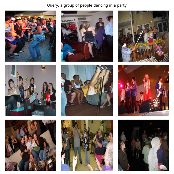
希望您喜歡這篇文章。對我來說,實施本文是一個非常有趣的經歷。我要感謝Khalid Salama提供了他提供的出色的Keras代碼示例,這激發了我在Pytorch中寫類似的東西。


